Author: Jason Brownlee
A learning curve is a plot of model learning performance over experience or time.
Learning curves are a widely used diagnostic tool in machine learning for algorithms that learn from a training dataset incrementally. The model can be evaluated on the training dataset and on a hold out validation dataset after each update during training and plots of the measured performance can created to show learning curves.
Reviewing learning curves of models during training can be used to diagnose problems with learning, such as an underfit or overfit model, as well as whether the training and validation datasets are suitably representative.
In this post, you will discover learning curves and how they can be used to diagnose the learning and generalization behavior of machine learning models, with example plots showing common learning problems.
After reading this post, you will know:
- Learning curves are plots that show changes in learning performance over time in terms of experience.
- Learning curves of model performance on the train and validation datasets can be used to diagnose an underfit, overfit, or well-fit model.
- Learning curves of model performance can be used to diagnose whether the train or validation datasets are not relatively representative of the problem domain.
Let’s get started.

A Gentle Introduction to Learning Curves for Diagnosing Deep Learning Model Performance
Photo by Mike Sutherland, some rights reserved.
Overview
This tutorial is divided into three parts; they are:
- Learning Curves
- Diagnosing Model Behavior
- Diagnosing Unrepresentative Datasets
Learning Curves in Machine Learning
Generally, a learning curve is a plot that shows time or experience on the x-axis and learning or improvement on the y-axis.
Learning curves (LCs) are deemed effective tools for monitoring the performance of workers exposed to a new task. LCs provide a mathematical representation of the learning process that takes place as task repetition occurs.
— Learning curve models and applications: Literature review and research directions, 2011.
For example, if you were learning a musical instrument, your skill on the instrument could be evaluated and assigned a numerical score each week for one year. A plot of the scores over the 52 weeks is a learning curve and would show how your learning of the instrument has changed over time.
- Learning Curve: Line plot of learning (y-axis) over experience (x-axis).
Learning curves are widely used in machine learning for algorithms that learn (optimize their internal parameters) incrementally over time, such as deep learning neural networks.
The metric used to evaluate learning could be maximizing, meaning that better scores (larger numbers) indicate more learning. An example would be classification accuracy.
It is more common to use a score that is minimizing, such as loss or error whereby better scores (smaller numbers) indicate more learning and a value of 0.0 indicates that the training dataset was learned perfectly and no mistakes were made.
During the training of a machine learning model, the current state of the model at each step of the training algorithm can be evaluated. It can be evaluated on the training dataset to give an idea of how well the model is “learning.” It can also be evaluated on a hold-out validation dataset that is not part of the training dataset. Evaluation on the validation dataset gives an idea of how well the model is “generalizing.”
- Train Learning Curve: Learning curve calculated from the training dataset that gives an idea of how well the model is learning.
- Validation Learning Curve: Learning curve calculated from a hold-out validation dataset that gives an idea of how well the model is generalizing.
It is common to create dual learning curves for a machine learning model during training on both the training and validation datasets.
In some cases, it is also common to create learning curves for multiple metrics, such as in the case of classification predictive modeling problems, where the model may be optimized according to cross-entropy loss and model performance is evaluated using classification accuracy. In this case, two plots are created, one for the learning curves of each metric, and each plot can show two learning curves, one for each of the train and validation datasets.
- Optimization Learning Curves: Learning curves calculated on the metric by which the parameters of the model are being optimized, e.g. loss.
- Performance Learning Curves: Learning curves calculated on the metric by which the model will be evaluated and selected, e.g. accuracy.
Now that we are familiar with the use of learning curves in machine learning, let’s look at some common shapes observed in learning curve plots.
Want Better Results with Deep Learning?
Take my free 7-day email crash course now (with sample code).
Click to sign-up and also get a free PDF Ebook version of the course.
Diagnosing Model Behavior
The shape and dynamics of a learning curve can be used to diagnose the behavior of a machine learning model and in turn perhaps suggest at the type of configuration changes that may be made to improve learning and/or performance.
There are three common dynamics that you are likely to observe in learning curves; they are:
- Underfit.
- Overfit.
- Good Fit.
We will take a closer look at each with examples. The examples will assume that we are looking at a minimizing metric, meaning that smaller relative scores on the y-axis indicate more or better learning.
Underfit Learning Curves
Underfitting refers to a model that cannot learn the training dataset.
Underfitting occurs when the model is not able to obtain a sufficiently low error value on the training set.
— Page 111, Deep Learning, 2016.
An underfit model can be identified from the learning curve of the training loss only.
It may show a flat line or noisy values of relatively high loss, indicating that the model was unable to learn the training dataset at all.
An example of this is provided below and is common when the model does not have a suitable capacity for the complexity of the dataset.
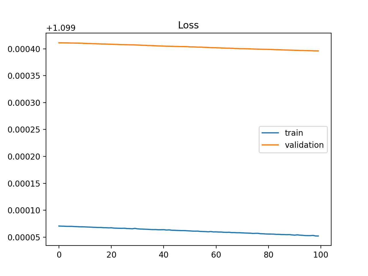
Example of Training Learning Curve Showing An Underfit Model That Does Not Have Sufficient Capacity
An underfit model may also be identified by a training loss that is decreasing and continues to decrease at the end of the plot.
This indicates that the model is capable of further learning and possible further improvements and that the training process was halted prematurely.
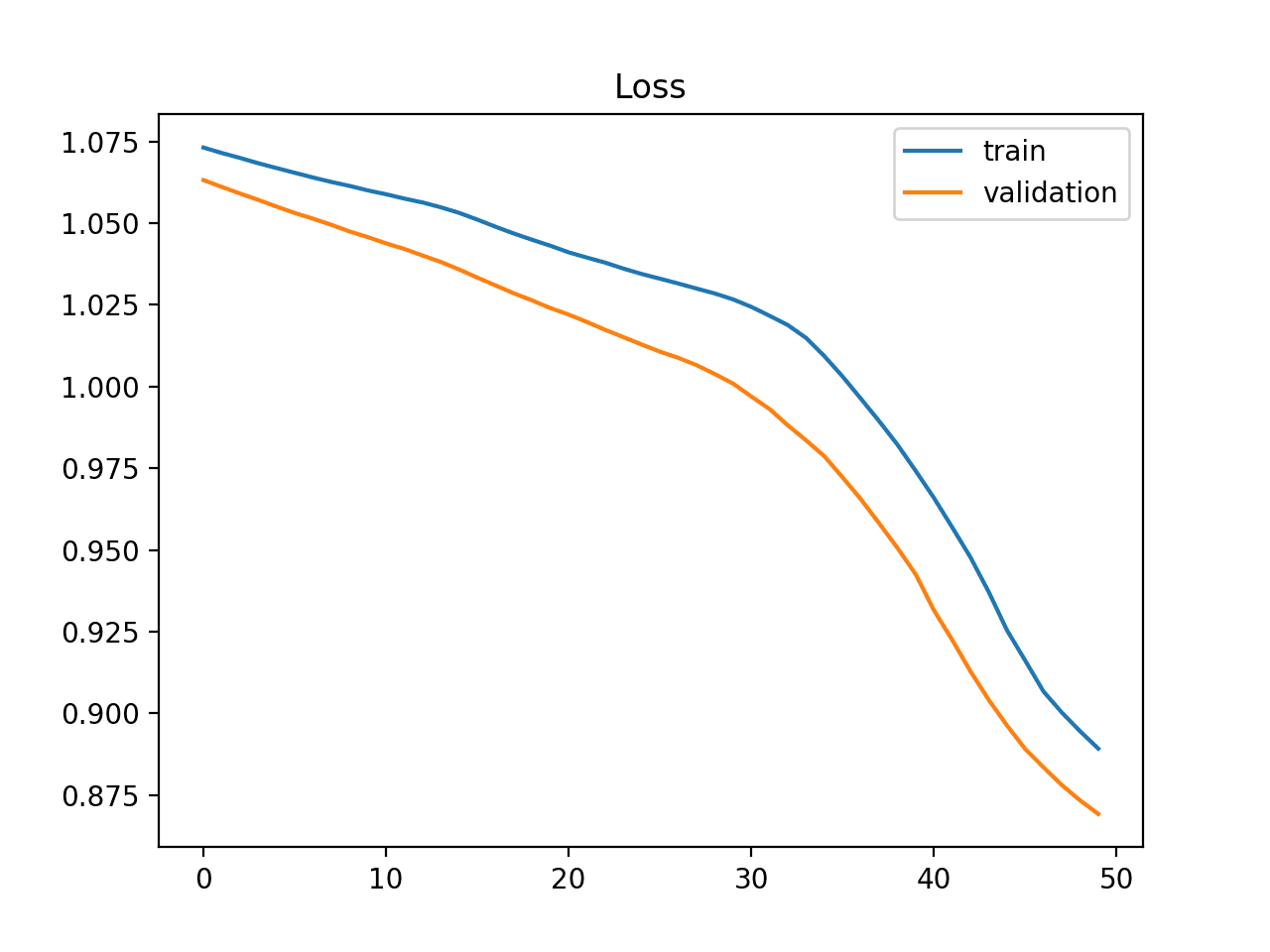
Example of Training Learning Curve Showing an Underfit Model That Requires Further Training
A plot of learning curves shows overfitting if:
- The training loss remains flat regardless of training.
- The training loss continues to decrease until the end of training.
Overfit Learning Curves
Overfitting refers to a model that has learned the training dataset too well, including the statistical noise or random fluctuations in the training dataset.
… fitting a more flexible model requires estimating a greater number of parameters. These more complex models can lead to a phenomenon known as overfitting the data, which essentially means they follow the errors, or noise, too closely.
— Page 22, An Introduction to Statistical Learning: with Applications in R, 2013.
The problem with overfitting, is that the more specialized the model becomes to training data, the less well it is able to generalize to new data, resulting in an increase in generalization error. This increase in generalization error can be measured by the performance of the model on the validation dataset.
This is an example of overfitting the data, […]. It is an undesirable situation because the fit obtained will not yield accurate estimates of the response on new observations that were not part of the original training data set.
— Page 24, An Introduction to Statistical Learning: with Applications in R, 2013.
This often occurs if the model has more capacity than is required for the problem, and, in turn, too much flexibility. It can also occur if the model is trained for too long.
A plot of learning curves shows overfitting if:
- The plot of training loss continues to decrease with experience.
- The plot of validation loss decreases to a point and begins increasing again.
The inflection point in validation loss may be the point at which training could be halted as experience after that point shows the dynamics of overfitting.
The example plot below demonstrates a case of overfitting.
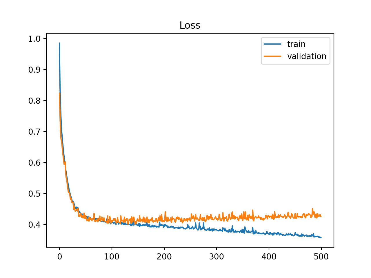
Example of Train and Validation Learning Curves Showing an Overfit Model
Good Fit Learning Curves
A good fit is the goal of the learning algorithm and exists between an overfit and underfit model.
A good fit is identified by a training and validation loss that decreases to a point of stability with a minimal gap between the two final loss values.
The loss of the model will almost always be lower on the training dataset than the validation dataset. This means that we should expect some gap between the train and validation loss learning curves. This gap is referred to as the “generalization gap.”
A plot of learning curves shows a good fit if:
- The plot of training loss decreases to a point of stability.
- The plot of validation loss decreases to a point of stability and has a small gap with the training loss.
Continued training of a good fit will likely lead to an overfit.
The example plot below demonstrates a case of a good fit.
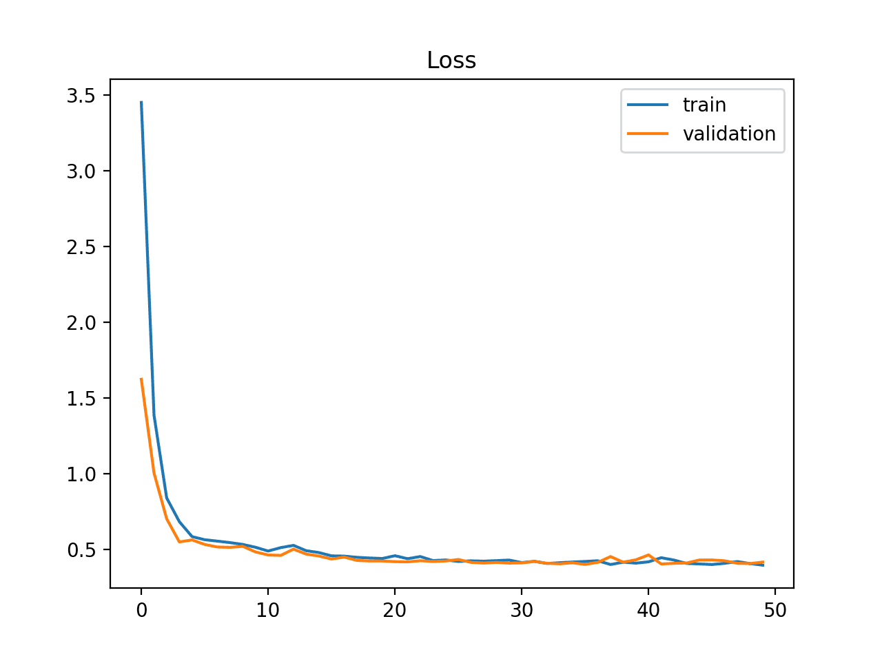
Example of Train and Validation Learning Curves Showing a Good Fit
Diagnosing Unrepresentative Datasets
Learning curves can also be used to diagnose properties of a dataset and whether it is relatively representative.
An unrepresentative dataset means a dataset that may not capture the statistical characteristics relative to another dataset drawn from the same domain, such as between a train and a validation dataset. This can commonly occur if the number of samples in a dataset is too small, relative to another dataset.
There are two common cases that could be observed; they are:
- Training dataset is relatively unrepresentative.
- Validation dataset is relatively unrepresentative.
Unrepresentative Train Dataset
An unrepresentative training dataset means that the training dataset does not provide sufficient information to learn the problem, relative to the validation dataset used to evaluate it.
This may occur if the training dataset has too few examples as compared to the validation dataset.
This situation can be identified by a learning curve for training loss that shows improvement and similarly a learning curve for validation loss that shows improvement, but a large gap remains between both curves.
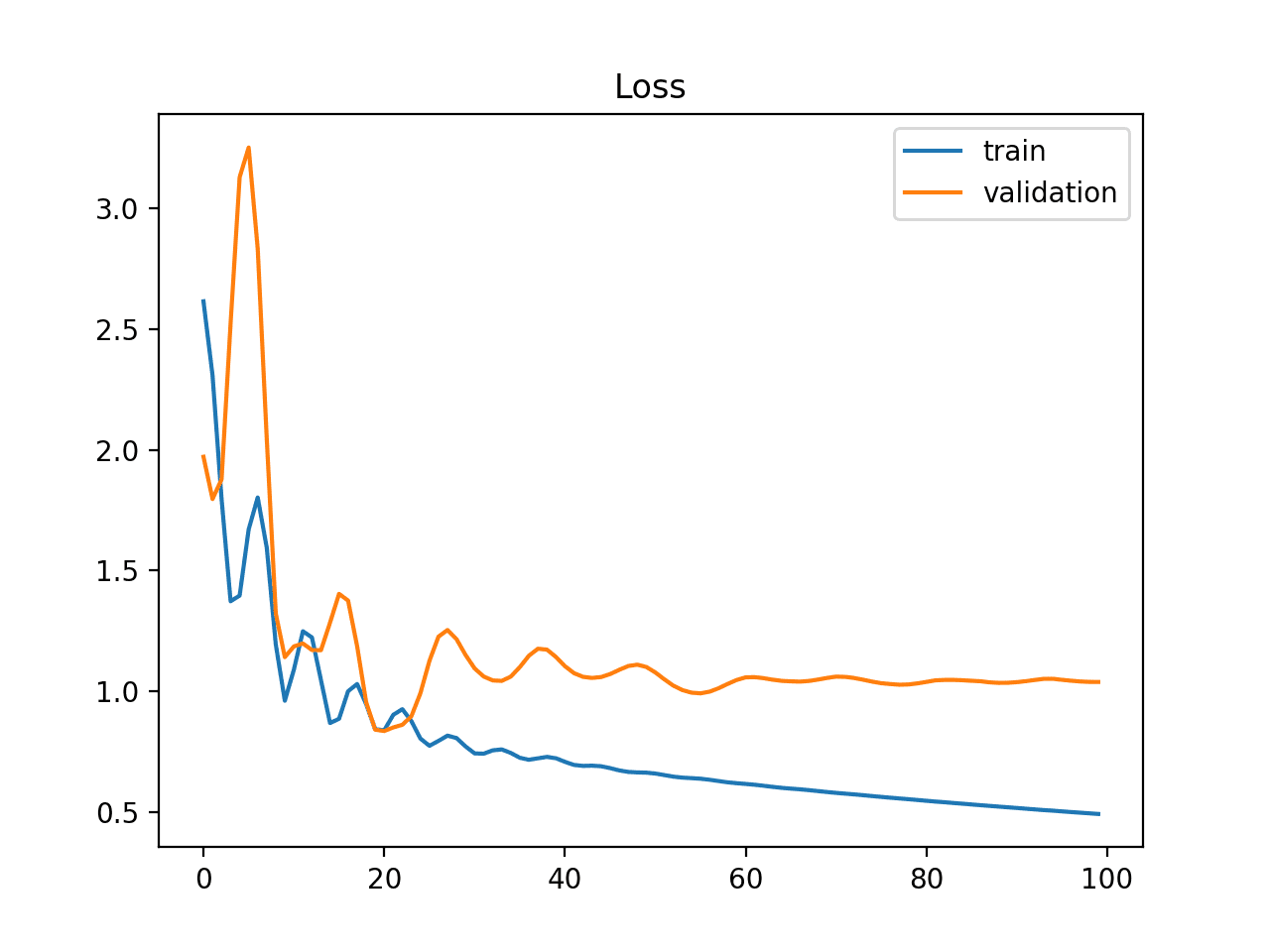
Example of Train and Validation Learning Curves Showing a Training Dataset That May Be too Small Relative to the Validation Dataset
Unrepresentative Validation Dataset
An unrepresentative validation dataset means that the validation dataset does not provide sufficient information to evaluate the ability of the model to generalize.
This may occur if the validation dataset has too few examples as compared to the training dataset.
This case can be identified by a learning curve for training loss that looks like a good fit (or other fits) and a learning curve for validation loss that shows noisy movements around the training loss.
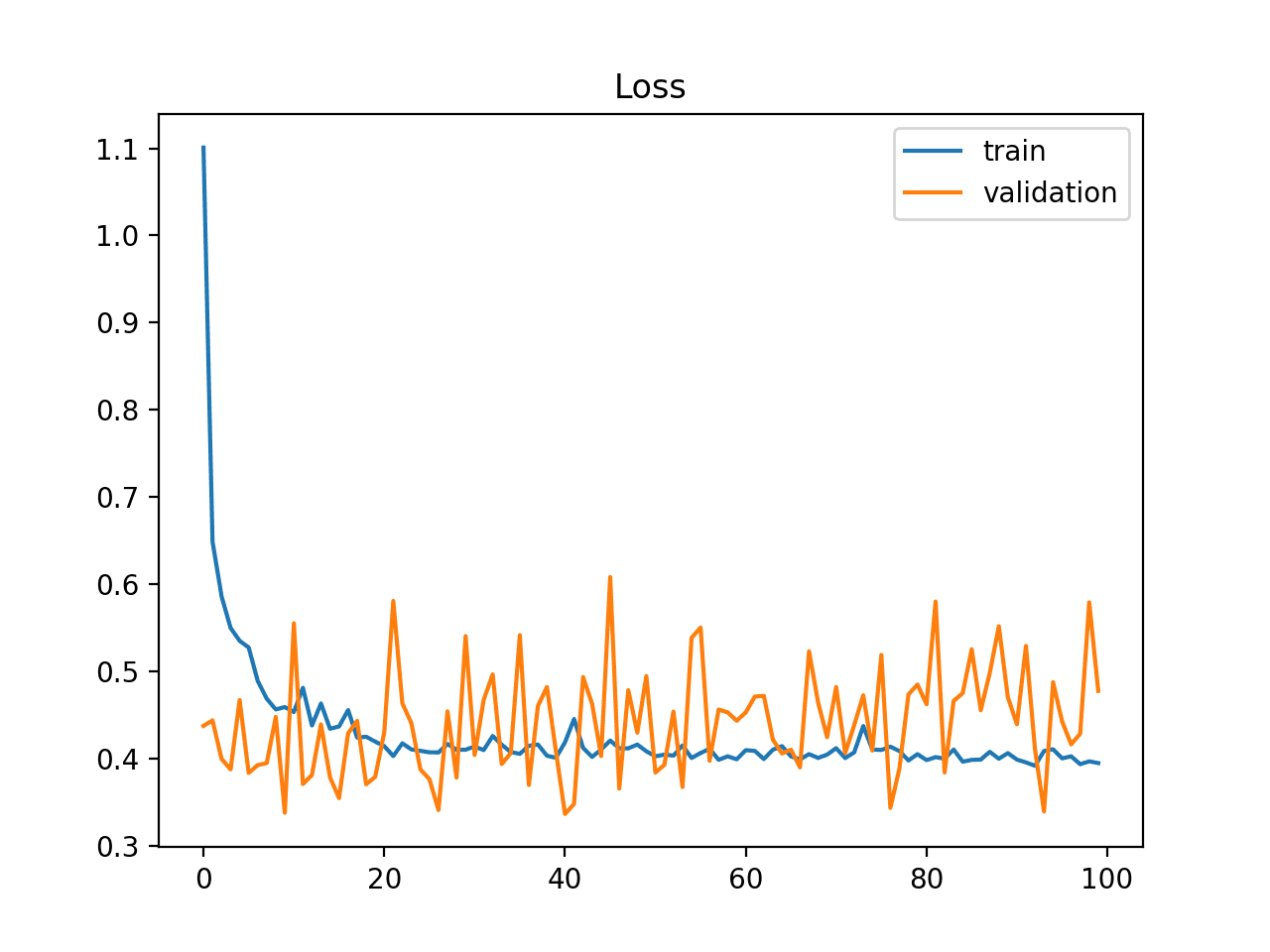
Example of Train and Validation Learning Curves Showing a Validation Dataset That May Be too Small Relative to the Training Dataset
It may also be identified by a validation loss that is lower than the training loss. In this case, it indicates that the validation dataset may be easier for the model to predict than the training dataset.
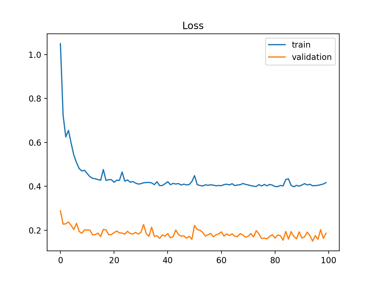
Example of Train and Validation Learning Curves Showing a Validation Dataset That Is Easier to Predict Than the Training Dataset
Further Reading
This section provides more resources on the topic if you are looking to go deeper.
Books
Papers
Posts
- How to Diagnose Overfitting and Underfitting of LSTM Models
- Overfitting and Underfitting With Machine Learning Algorithms
Articles
Summary
In this post, you discovered learning curves and how they can be used to diagnose the learning and generalization behavior of machine learning models.
Specifically, you learned:
- Learning curves are plots that show changes in learning performance over time in terms of experience.
- Learning curves of model performance on the train and validation datasets can be used to diagnose an underfit, overfit, or well-fit model.
- Learning curves of model performance can be used to diagnose whether the train or validation datasets are not relatively representative of the problem domain.
Do you have any questions?
Ask your questions in the comments below and I will do my best to answer.
The post A Gentle Introduction to Learning Curves for Diagnosing Machine Learning Model Performance appeared first on Machine Learning Mastery.
