Author: Jason Brownlee
Deep learning neural networks are generally opaque, meaning that although they can make useful and skillful predictions, it is not clear how or why a given prediction was made.
Convolutional neural networks, have internal structures that are designed to operate upon two-dimensional image data, and as such preserve the spatial relationships for what was learned by the model. Specifically, the two-dimensional filters learned by the model can be inspected and visualized to discover the types of features that the model will detect, and the activation maps output by convolutional layers can be inspected to understand exactly what features were detected for a given input image.
In this tutorial, you will discover how to develop simple visualizations for filters and feature maps in a convolutional neural network.
After completing this tutorial, you will know:
- How to develop a visualization for specific filters in a convolutional neural network.
- How to develop a visualization for specific feature maps in a convolutional neural network.
- How to systematically visualize feature maps for each block in a deep convolutional neural network.
Let’s get started.
How to Visualize Filters and Feature Maps in Convolutional Neural Networks
Photo by Mark Kent, some rights reserved.
Tutorial Overview
This tutorial is divided into four parts; they are:
- Visualizing Convolutional Layers
- Pre-fit VGG Model
- How to Visualize Filters
- How to Visualize Feature Maps
Visualizing Convolutional Layers
Neural network models are generally referred to as being opaque. This means that they are poor at explaining the reason why a specific decision or prediction was made.
Convolutional neural networks are designed to work with image data, and their structure and function suggest that should be less inscrutable than other types of neural networks.
Specifically, the models are comprised of small linear filters and the result of applying filters called activation maps, or more generally, feature maps.
Both filters and feature maps can be visualized.
For example, we can design and understand small filters, such as line detectors. Perhaps visualizing the filters within a learned convolutional neural network can provide insight into how the model works.
The feature maps that result from applying filters to input images and to feature maps output by prior layers could provide insight into the internal representation that the model has of a specific input at a given point in the model.
We will explore both of these approaches to visualizing a convolutional neural network in this tutorial.
Want Results with Deep Learning for Computer Vision?
Take my free 7-day email crash course now (with sample code).
Click to sign-up and also get a free PDF Ebook version of the course.
Pre-fit VGG Model
We need a model to visualize.
Instead of fitting a model from scratch, we can use a pre-fit prior state-of-the-art image classification model.
Keras provides many examples of well-performing image classification models developed by different research groups for the ImageNet Large Scale Visual Recognition Challenge, or ILSVRC. One example is the VGG-16 model that achieved top results in the 2014 competition.
This is a good model to use for visualization because it has a simple uniform structure of serially ordered convolutional and pooling layers, it is deep with 16 learned layers, and it performed very well, meaning that the filters and resulting feature maps will capture useful features. For more information on this model, see the 2015 paper “Very Deep Convolutional Networks for Large-Scale Image Recognition.”
We can load and summarize the VGG16 model with just a few lines of code; for example:
# load vgg model
from keras.applications.vgg16 import VGG16
# load the model
model = VGG16()
# summarize the model
model.summary()
Running the example will load the model weights into memory and print a summary of the loaded model.
If this is the first time that you have loaded the model, the weights will be downloaded from the internet and stored in your home directory. These weights are approximately 500 megabytes and may take a moment to download depending on the speed of your internet connection.
We can see that the layers are well named, organized into blocks, and named with integer indexes within each block.
_________________________________________________________________
Layer (type)                 Output Shape              Param #
=================================================================
input_1 (InputLayer)         (None, 224, 224, 3)       0
_________________________________________________________________
block1_conv1 (Conv2D)        (None, 224, 224, 64)      1792
_________________________________________________________________
block1_conv2 (Conv2D)        (None, 224, 224, 64)      36928
_________________________________________________________________
block1_pool (MaxPooling2D)   (None, 112, 112, 64)      0
_________________________________________________________________
block2_conv1 (Conv2D)        (None, 112, 112, 128)     73856
_________________________________________________________________
block2_conv2 (Conv2D)        (None, 112, 112, 128)     147584
_________________________________________________________________
block2_pool (MaxPooling2D)   (None, 56, 56, 128)       0
_________________________________________________________________
block3_conv1 (Conv2D)        (None, 56, 56, 256)       295168
_________________________________________________________________
block3_conv2 (Conv2D)        (None, 56, 56, 256)       590080
_________________________________________________________________
block3_conv3 (Conv2D)        (None, 56, 56, 256)       590080
_________________________________________________________________
block3_pool (MaxPooling2D)   (None, 28, 28, 256)       0
_________________________________________________________________
block4_conv1 (Conv2D)        (None, 28, 28, 512)       1180160
_________________________________________________________________
block4_conv2 (Conv2D)        (None, 28, 28, 512)       2359808
_________________________________________________________________
block4_conv3 (Conv2D)        (None, 28, 28, 512)       2359808
_________________________________________________________________
block4_pool (MaxPooling2D)   (None, 14, 14, 512)       0
_________________________________________________________________
block5_conv1 (Conv2D)        (None, 14, 14, 512)       2359808
_________________________________________________________________
block5_conv2 (Conv2D)        (None, 14, 14, 512)       2359808
_________________________________________________________________
block5_conv3 (Conv2D)        (None, 14, 14, 512)       2359808
_________________________________________________________________
block5_pool (MaxPooling2D)   (None, 7, 7, 512)         0
_________________________________________________________________
flatten (Flatten)            (None, 25088)             0
_________________________________________________________________
fc1 (Dense)                  (None, 4096)              102764544
_________________________________________________________________
fc2 (Dense)                  (None, 4096)              16781312
_________________________________________________________________
predictions (Dense)          (None, 1000)              4097000
=================================================================
Total params: 138,357,544
Trainable params: 138,357,544
Non-trainable params: 0
_________________________________________________________________
Now that we have a pre-fit model, we can use it as the basis for visualizations.
How to Visualize Filters
Perhaps the simplest visualization to perform is to plot the learned filters directly.
In neural network terminology, the learned filters are simply weights, yet because of the specialized two-dimensional structure of the filters, the weight values have a spatial relationship to each other and plotting each filter as a two-dimensional image is meaningful (or could be).
The first step is to review the filters in the model, to see what we have to work with.
The model summary printed in the previous section summarizes the output shape of each layer, e.g. the shape of the resulting feature maps. It does not give any idea of the shape of the filters (weights) in the network, only the total number of weights per layer.
We can access all of the layers of the model via the model.layers property.
Each layer has a layer.name property, where the convolutional layers have a naming convolution like block#_conv#, where the ‘#‘ is an integer. Therefore, we can check the name of each layer and skip any that don’t contain the string ‘conv‘.
# summarize filter shapes
for layer in model.layers:
	# check for convolutional layer
	if 'conv' not in layer.name:
		continue
Each convolutional layer has two sets of weights.
One is the block of filters and the other is the block of bias values. These are accessible via the layer.get_weights() function. We can retrieve these weights and then summarize their shape.
# get filter weights
filters, biases = layer.get_weights()
print(layer.name, filters.shape)
Tying this together, the complete example of summarizing the model filters is listed below.
# summarize filters in each convolutional layer
from keras.applications.vgg16 import VGG16
from matplotlib import pyplot
# load the model
model = VGG16()
# summarize filter shapes
for layer in model.layers:
	# check for convolutional layer
	if 'conv' not in layer.name:
		continue
	# get filter weights
	filters, biases = layer.get_weights()
	print(layer.name, filters.shape)
Running the example prints a list of layer details including the layer name and the shape of the filters in the layer.
block1_conv1 (3, 3, 3, 64)
block1_conv2 (3, 3, 64, 64)
block2_conv1 (3, 3, 64, 128)
block2_conv2 (3, 3, 128, 128)
block3_conv1 (3, 3, 128, 256)
block3_conv2 (3, 3, 256, 256)
block3_conv3 (3, 3, 256, 256)
block4_conv1 (3, 3, 256, 512)
block4_conv2 (3, 3, 512, 512)
block4_conv3 (3, 3, 512, 512)
block5_conv1 (3, 3, 512, 512)
block5_conv2 (3, 3, 512, 512)
block5_conv3 (3, 3, 512, 512)
We can see that all convolutional layers use 3×3 filters, which are small and perhaps easy to interpret.
An architectural concern with a convolutional neural network is that the depth of a filter must match the depth of the input for the filter (e.g. the number of channels).
We can see that for the input image with three channels for red, green and blue, that each filter has a depth of three (here we are working with a channel-last format). We could visualize one filter as a plot with three images, one for each channel, or compress all three down to a single color image, or even just look at the first channel and assume the other channels will look the same. The problem is, we then have 63 other filters that we might like to visualize.
We can retrieve the filters from the first layer as follows:
# retrieve weights from the second hidden layer
filters, biases = model.layers[1].get_weights()
The weight values will likely be small positive and negative values centered around 0.0.
We can normalize their values to the range 0-1 to make them easy to visualize.
# normalize filter values to 0-1 so we can visualize them
f_min, f_max = filters.min(), filters.max()
filters = (filters - f_min) / (f_max - f_min)
Now we can enumerate the first six filters out of the 64 in the block and plot each of the three channels of each filter.
We use the matplotlib library and plot each filter as a new row of subplots, and each filter channel or depth as a new column.
# plot first few filters
n_filters, ix = 6, 1
for i in range(n_filters):
	# get the filter
	f = filters[:, :, :, i]
	# plot each channel separately
	for j in range(3):
		# specify subplot and turn of axis
		ax = pyplot.subplot(n_filters, 3, ix)
		ax.set_xticks([])
		ax.set_yticks([])
		# plot filter channel in grayscale
		pyplot.imshow(f[:, :, j], cmap='gray')
		ix += 1
# show the figure
pyplot.show()
Tying this together, the complete example of plotting the first six filters from the first hidden convolutional layer in the VGG16 model is listed below.
# cannot easily visualize filters lower down
from keras.applications.vgg16 import VGG16
from matplotlib import pyplot
# load the model
model = VGG16()
# retrieve weights from the second hidden layer
filters, biases = model.layers[1].get_weights()
# normalize filter values to 0-1 so we can visualize them
f_min, f_max = filters.min(), filters.max()
filters = (filters - f_min) / (f_max - f_min)
# plot first few filters
n_filters, ix = 6, 1
for i in range(n_filters):
	# get the filter
	f = filters[:, :, :, i]
	# plot each channel separately
	for j in range(3):
		# specify subplot and turn of axis
		ax = pyplot.subplot(n_filters, 3, ix)
		ax.set_xticks([])
		ax.set_yticks([])
		# plot filter channel in grayscale
		pyplot.imshow(f[:, :, j], cmap='gray')
		ix += 1
# show the figure
pyplot.show()
Running the example creates a figure with six rows of three images, or 18 images, one row for each filter and one column for each channel
We can see that in some cases, the filter is the same across the channels (the first row), and in others, the filters differ (the last row).
The dark squares indicate small or inhibitory weights and the light squares represent large or excitatory weights. Using this intuition, we can see that the filters on the first row detect a gradient from light in the top left to dark in the bottom right.
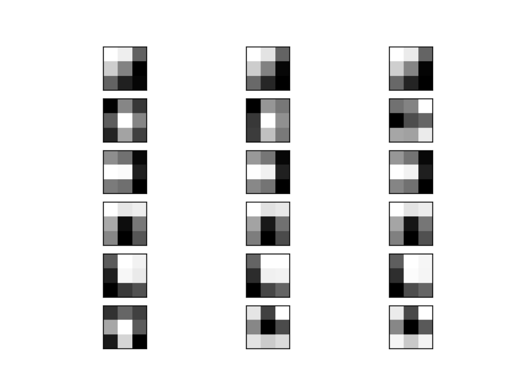
Plot of the First 6 Filters From VGG16 With One Subplot per Channel
Although we have a visualization, we only see the first six of the 64 filters in the first convolutional layer. Visualizing all 64 filters in one image is feasible.
Sadly, this does not scale; if we wish to start looking at filters in the second convolutional layer, we can see that again we have 64 filters, but each has 64 channels to match the input feature maps. To see all 64 channels in a row for all 64 filters would require (64×64) 4,096 subplots in which it may be challenging to see any detail.
How to Visualize Feature Maps
The activation maps, called feature maps, capture the result of applying the filters to input, such as the input image or another feature map.
The idea of visualizing a feature map for a specific input image would be to understand what features of the input are detected or preserved in the feature maps. The expectation would be that the feature maps close to the input detect small or fine-grained detail, whereas feature maps close to the output of the model capture more general features.
In order to explore the visualization of feature maps, we need input for the VGG16 model that can be used to create activations. We will use a simple photograph of a bird. Specifically, a Robin, taken by Chris Heald and released under a permissive license.
Download the photograph and place it in your current working directory with the filename ‘bird.jpg‘.

Robin, by Chris Heald
Next, we need a clearer idea of the shape of the feature maps output by each of the convolutional layers and the layer index number so that we can retrieve the appropriate layer output.
The example below will enumerate all layers in the model and print the output size or feature map size for each convolutional layer as well as the layer index in the model.
# summarize feature map size for each conv layer
from keras.applications.vgg16 import VGG16
from matplotlib import pyplot
# load the model
model = VGG16()
# summarize feature map shapes
for i in range(len(model.layers)):
	layer = model.layers[i]
	# check for convolutional layer
	if 'conv' not in layer.name:
		continue
	# summarize output shape
	print(i, layer.name, layer.output.shape)
Running the example, we see the same output shapes as we saw in the model summary, but in this case only for the convolutional layers.
1 block1_conv1 (?, 224, 224, 64)
2 block1_conv2 (?, 224, 224, 64)
4 block2_conv1 (?, 112, 112, 128)
5 block2_conv2 (?, 112, 112, 128)
7 block3_conv1 (?, 56, 56, 256)
8 block3_conv2 (?, 56, 56, 256)
9 block3_conv3 (?, 56, 56, 256)
11 block4_conv1 (?, 28, 28, 512)
12 block4_conv2 (?, 28, 28, 512)
13 block4_conv3 (?, 28, 28, 512)
15 block5_conv1 (?, 14, 14, 512)
16 block5_conv2 (?, 14, 14, 512)
17 block5_conv3 (?, 14, 14, 512)
We can use this information and design a new model that is a subset of the layers in the full VGG16 model. The model would have the same input layer as the original model, but the output would be the output of a given convolutional layer, which we know would be the activation of the layer or the feature map.
For example, after loading the VGG model, we can define a new model that outputs a feature map from the first convolutional layer (index 1) as follows.
# redefine model to output right after the first hidden layer
model = Model(inputs=model.inputs, outputs=model.layers[1].output)
Making a prediction with this model will give the feature map for the first convolutional layer for a given provided input image. Let’s implement this.
After defining the model, we need to load the bird image with the size expected by the model, in this case, 224×224.
# load the image with the required shape
img = load_img('bird.jpg', target_size=(224, 224))
Next, the image PIL object needs to be converted to a NumPy array of pixel data and expanded from a 3D array to a 4D array with the dimensions of [samples, rows, cols, channels], where we only have one sample.
# convert the image to an array
img = img_to_array(img)
# expand dimensions so that it represents a single 'sample'
img = expand_dims(img, axis=0)
The pixel values then need to be scaled appropriately for the VGG model.
# prepare the image (e.g. scale pixel values for the vgg)
img = preprocess_input(img)
We are now ready to get the feature map. We can do this easy by calling the model.predict() function and passing in the prepared single image.
# get feature map for first hidden layer
feature_maps = model.predict(img)
We know the result will be a feature map with 224x224x64. We can plot all 64 two-dimensional images as an 8×8 square of images.
# plot all 64 maps in an 8x8 squares
square = 8
ix = 1
for _ in range(square):
	for _ in range(square):
		# specify subplot and turn of axis
		ax = pyplot.subplot(square, square, ix)
		ax.set_xticks([])
		ax.set_yticks([])
		# plot filter channel in grayscale
		pyplot.imshow(feature_maps[0, :, :, ix-1], cmap='gray')
		ix += 1
# show the figure
pyplot.show()
Tying all of this together, the complete code example of visualizing the feature map for the first convolutional layer in the VGG16 model for a bird input image is listed below.
# plot feature map of first conv layer for given image
from keras.applications.vgg16 import VGG16
from keras.applications.vgg16 import preprocess_input
from keras.preprocessing.image import load_img
from keras.preprocessing.image import img_to_array
from keras.models import Model
from matplotlib import pyplot
from numpy import expand_dims
# load the model
model = VGG16()
# redefine model to output right after the first hidden layer
model = Model(inputs=model.inputs, outputs=model.layers[1].output)
model.summary()
# load the image with the required shape
img = load_img('bird.jpg', target_size=(224, 224))
# convert the image to an array
img = img_to_array(img)
# expand dimensions so that it represents a single 'sample'
img = expand_dims(img, axis=0)
# prepare the image (e.g. scale pixel values for the vgg)
img = preprocess_input(img)
# get feature map for first hidden layer
feature_maps = model.predict(img)
# plot all 64 maps in an 8x8 squares
square = 8
ix = 1
for _ in range(square):
	for _ in range(square):
		# specify subplot and turn of axis
		ax = pyplot.subplot(square, square, ix)
		ax.set_xticks([])
		ax.set_yticks([])
		# plot filter channel in grayscale
		pyplot.imshow(feature_maps[0, :, :, ix-1], cmap='gray')
		ix += 1
# show the figure
pyplot.show()
Running the example first summarizes the new, smaller model that takes an image and outputs a feature map.
Remember: this model is much smaller than the VGG16 model, but still uses the same weights (filters) in the first convolutional layer as the VGG16 model.
_________________________________________________________________
Layer (type)                 Output Shape              Param #
=================================================================
input_1 (InputLayer)         (None, 224, 224, 3)       0
_________________________________________________________________
block1_conv1 (Conv2D)        (None, 224, 224, 64)      1792
=================================================================
Total params: 1,792
Trainable params: 1,792
Non-trainable params: 0
_________________________________________________________________
Next, a figure is created that shows all 64 feature maps as subplots.
We can see that the result of applying the filters in the first convolutional layer is a lot of versions of the bird image with different features highlighted.
For example, some highlight lines, other focus on the background or the foreground.
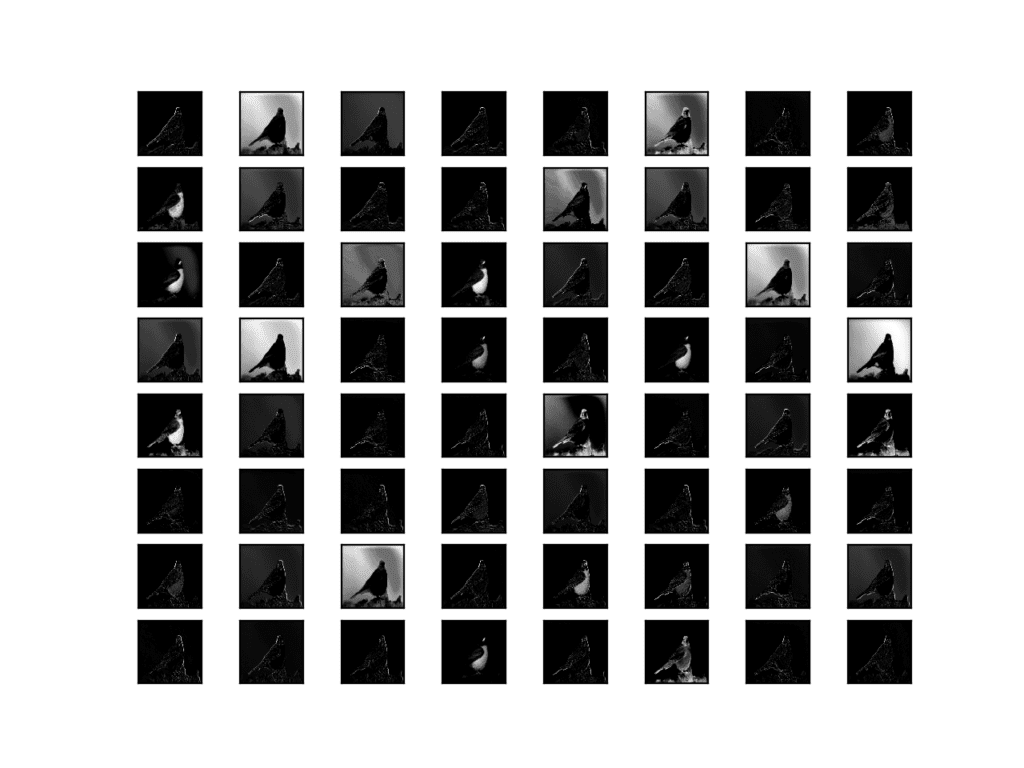
Visualization of the Feature Maps Extracted From the First Convolutional Layer in the VGG16 Model
This is an interesting result and generally matches our expectation. We could update the example to plot the feature maps from the output of other specific convolutional layers.
Another approach would be to collect feature maps output from each block of the model in a single pass, then create an image of each.
There are five main blocks in the image (e.g. block1, block2, etc.) that end in a pooling layer. The layer indexes of the last convolutional layer in each block are [2, 5, 9, 13, 17].
We can define a new model that has multiple outputs, one feature map output for each of the last convolutional layer in each block; for example:
# redefine model to output right after the first hidden layer
ixs = [2, 5, 9, 13, 17]
outputs = [model.layers[i+1].output for i in ixs]
model = Model(inputs=model.inputs, outputs=outputs)
model.summary()
Making a prediction with this new model will result in a list of feature maps.
We know that the number of feature maps (e.g. depth or number of channels) in deeper layers is much more than 64, such as 256 or 512. Nevertheless, we can cap the number of feature maps visualized at 64 for consistency.
# plot the output from each block
square = 8
for fmap in feature_maps:
	# plot all 64 maps in an 8x8 squares
	ix = 1
	for _ in range(square):
		for _ in range(square):
			# specify subplot and turn of axis
			ax = pyplot.subplot(square, square, ix)
			ax.set_xticks([])
			ax.set_yticks([])
			# plot filter channel in grayscale
			pyplot.imshow(fmap[0, :, :, ix-1], cmap='gray')
			ix += 1
	# show the figure
	pyplot.show()
Tying these changes together, we can now create five separate plots for each of the five blocks in the VGG16 model for our bird photograph. The complete listing is provided below.
# visualize feature maps output from each block in the vgg model
from keras.applications.vgg16 import VGG16
from keras.applications.vgg16 import preprocess_input
from keras.preprocessing.image import load_img
from keras.preprocessing.image import img_to_array
from keras.models import Model
from matplotlib import pyplot
from numpy import expand_dims
# load the model
model = VGG16()
# redefine model to output right after the first hidden layer
ixs = [2, 5, 9, 13, 17]
outputs = [model.layers[i].output for i in ixs]
model = Model(inputs=model.inputs, outputs=outputs)
# load the image with the required shape
img = load_img('bird.jpg', target_size=(224, 224))
# convert the image to an array
img = img_to_array(img)
# expand dimensions so that it represents a single 'sample'
img = expand_dims(img, axis=0)
# prepare the image (e.g. scale pixel values for the vgg)
img = preprocess_input(img)
# get feature map for first hidden layer
feature_maps = model.predict(img)
# plot the output from each block
square = 8
for fmap in feature_maps:
	# plot all 64 maps in an 8x8 squares
	ix = 1
	for _ in range(square):
		for _ in range(square):
			# specify subplot and turn of axis
			ax = pyplot.subplot(square, square, ix)
			ax.set_xticks([])
			ax.set_yticks([])
			# plot filter channel in grayscale
			pyplot.imshow(fmap[0, :, :, ix-1], cmap='gray')
			ix += 1
	# show the figure
	pyplot.show()
Running the example results in five plots showing the feature maps from the five main blocks of the VGG16 model.
We can see that the feature maps closer to the input of the model capture a lot of fine detail in the image and that as we progress deeper into the model, the feature maps show less and less detail.
This pattern was to be expected, as the model abstracts the features from the image into more general concepts that can be used to make a classification. Although it is not clear from the final image that the model saw a bird, we generally lose the ability to interpret these deeper feature maps.
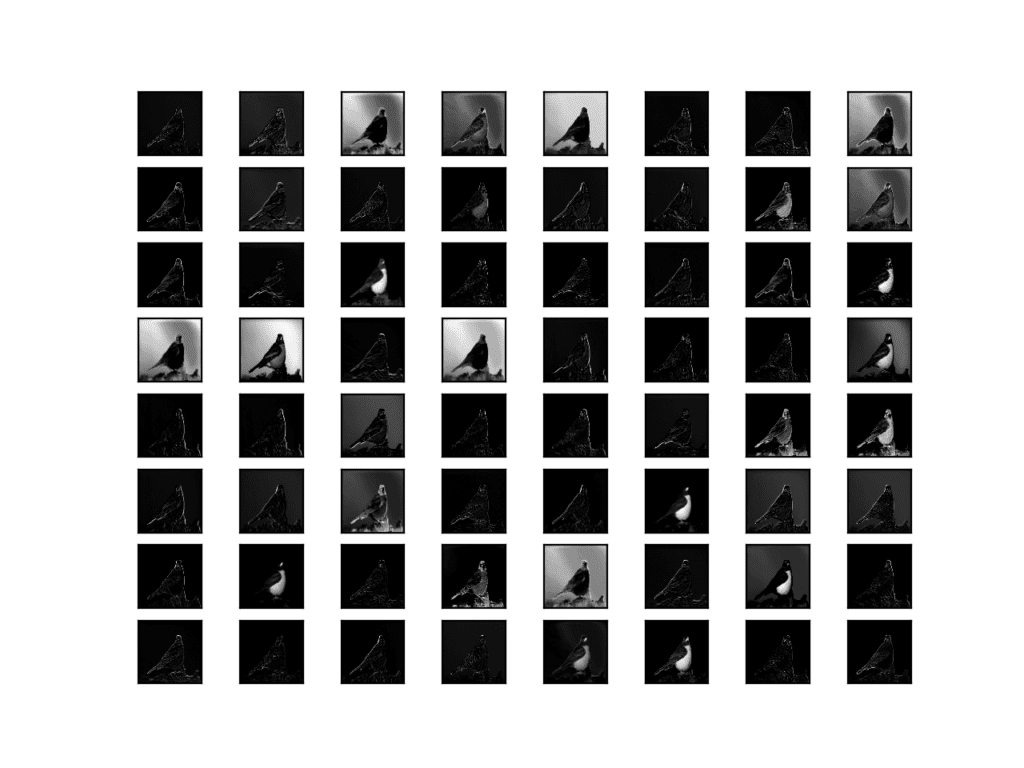
Visualization of the Feature Maps Extracted From Block 1 in the VGG16 Model
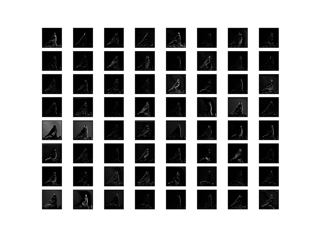
Visualization of the Feature Maps Extracted From Block 2 in the VGG16 Model
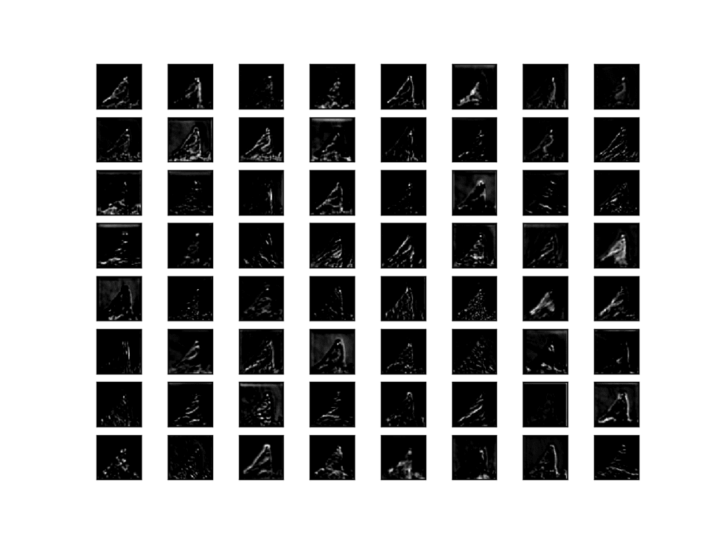
Visualization of the Feature Maps Extracted From Block 3 in the VGG16 Model
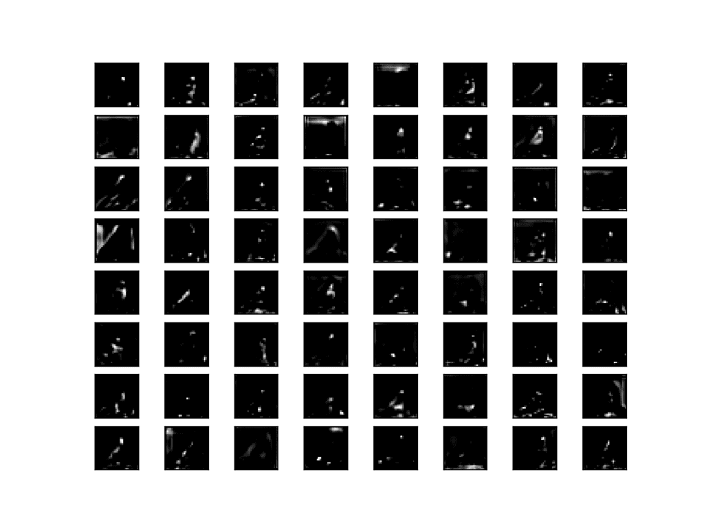
Visualization of the Feature Maps Extracted From Block 4 in the VGG16 Model
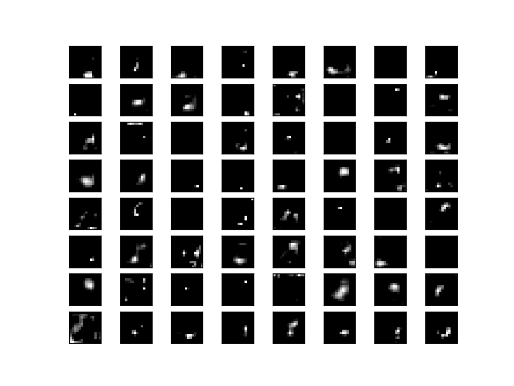
Visualization of the Feature Maps Extracted From Block 5 in the VGG16 Model
Further Reading
This section provides more resources on the topic if you are looking to go deeper.
Books
- Chapter 9: Convolutional Networks, Deep Learning, 2016.
- Chapter 5: Deep Learning for Computer Vision, Deep Learning with Python, 2017.
API
Articles
- Lecture 12 | Visualizing and Understanding, CS231n: Convolutional Neural Networks for Visual Recognition, (slides) 2017.
- Visualizing what ConvNets learn, CS231n: Convolutional Neural Networks for Visual Recognition.
- How convolutional neural networks see the world, 2016.
Summary
In this tutorial, you discovered how to develop simple visualizations for filters and feature maps in a convolutional neural network.
Specifically, you learned:
- How to develop a visualization for specific filters in a convolutional neural network.
- How to develop a visualization for specific feature maps in a convolutional neural network.
- How to systematically visualize feature maps for each block in a deep convolutional neural network.
Do you have any questions?
Ask your questions in the comments below and I will do my best to answer.
The post How to Visualize Filters and Feature Maps in Convolutional Neural Networks appeared first on Machine Learning Mastery.
