How to Develop a 1D Generative Adversarial Network From Scratch in Keras

Author: Jason Brownlee

Generative Adversarial Networks, or GANs for short, are a deep learning architecture for training powerful generator models.

A generator model is capable of generating new artificial samples that plausibly could have come from an existing distribution of samples.

GANs are comprised of both generator and discriminator models. The generator is responsible for generating new samples from the domain, and the discriminator is responsible for classifying whether samples are real or fake (generated). Importantly, the performance of the discriminator model is used to update both the model weights of the discriminator itself and the generator model. This means that the generator never actually sees examples from the domain and is adapted based on how well the discriminator performs.

This is a complex type of model both to understand and to train.

One approach to better understand the nature of GAN models and how they can be trained is to develop a model from scratch for a very simple task.

A simple task that provides a good context for developing a simple GAN from scratch is a one-dimensional function. This is because both real and generated samples can be plotted and visually inspected to get an idea of what has been learned. A simple function also does not require sophisticated neural network models, meaning the specific generator and discriminator models used on the architecture can be easily understood.

In this tutorial, we will select a simple one-dimensional function and use it as the basis for developing and evaluating a generative adversarial network from scratch using the Keras deep learning library.

After completing this tutorial, you will know:

The benefit of developing a generative adversarial network from scratch for a simple one-dimensional function.
How to develop separate discriminator and generator models, as well as a composite model for training the generator via the discriminator’s predictive behavior.
How to subjectively evaluate generated samples in the context of real examples from the problem domain.

Let’s get started.

How to Develop a Generative Adversarial Network for a 1-Dimensional Function From Scratch in Keras
Photo by Chris Bambrick, some rights reserved.

Tutorial Overview

This tutorial is divided into six parts; they are:

Select a One-Dimensional Function
Define a Discriminator Model
Define a Generator Model
Training the Generator Model
Evaluating the Performance of the GAN
Complete Example of Training the GAN

Select a One-Dimensional Function

The first step is to select a one-dimensional function to model.

Something of the form:

y = f(x)

Where x are input values and y are the output values of the function.

Specifically, we want a function that we can easily understand and plot. This will help in both setting an expectation of what the model should be generating and in using a visual inspection of generated examples to get an idea of their quality.

We will use a simple function of x^2; that is, the function will return the square of the input. You might remember this function from high school algebra as the u-shaped function.

We can define the function in Python as follows:

# simple function
def calculate(x):
	return x * x

We can define the input domain as real values between -0.5 and 0.5 and calculate the output value for each input value in this linear range, then plot the results to get an idea of how inputs relate to outputs.

The complete example is listed below.

# demonstrate simple x^2 function
from matplotlib import pyplot

# simple function
def calculate(x):
	return x * x

# define inputs
inputs = [-0.5, -0.4, -0.3, -0.2, -0.1, 0, 0.1, 0.2, 0.3, 0.4, 0.5]
# calculate outputs
outputs = [calculate(x) for x in inputs]
# plot the result
pyplot.plot(inputs, outputs)
pyplot.show()

Running the example calculates the output value for each input value and creates a plot of input vs. output values.

We can see that values far from 0.0 result in larger output values, whereas values close to zero result in smaller output values, and that this behavior is symmetrical around zero.

This is the well-known u-shape plot of the X^2 one-dimensional function.

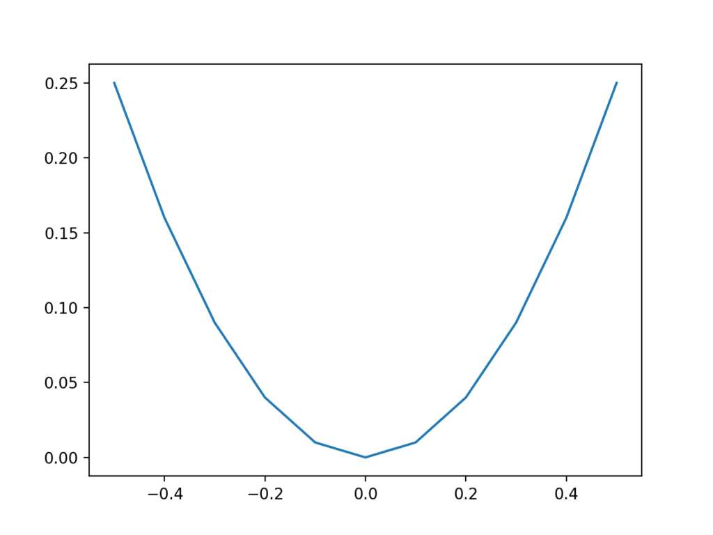
Plot of inputs vs. outputs for X^2 function.

We can generate random samples or points from the function.

This can be achieved by generating random values between -0.5 and 0.5 and calculating the associated output value. Repeating this many times will give a sample of points from the function, e.g. “real samples.”

Plotting these samples using a scatter plot will show the same u-shape plot, although comprised of the individual random samples.

The complete example is listed below.

First, we generate uniformly random values between 0 and 1, then shift them to the range -0.5 and 0.5. We then calculate the output value for each randomly generated input value and combine the arrays into a single NumPy array with n rows (100) and two columns.

# example of generating random samples from X^2
from numpy.random import rand
from numpy import hstack
from matplotlib import pyplot

# generate randoms sample from x^2
def generate_samples(n=100):
	# generate random inputs in [-0.5, 0.5]
	X1 = rand(n) - 0.5
	# generate outputs X^2 (quadratic)
	X2 = X1 * X1
	# stack arrays
	X1 = X1.reshape(n, 1)
	X2 = X2.reshape(n, 1)
	return hstack((X1, X2))

# generate samples
data = generate_samples()
# plot samples
pyplot.scatter(data[:, 0], data[:, 1])
pyplot.show()

Running the example generates 100 random inputs and their calculated output and plots the sample as a scatter plot, showing the familiar u-shape.

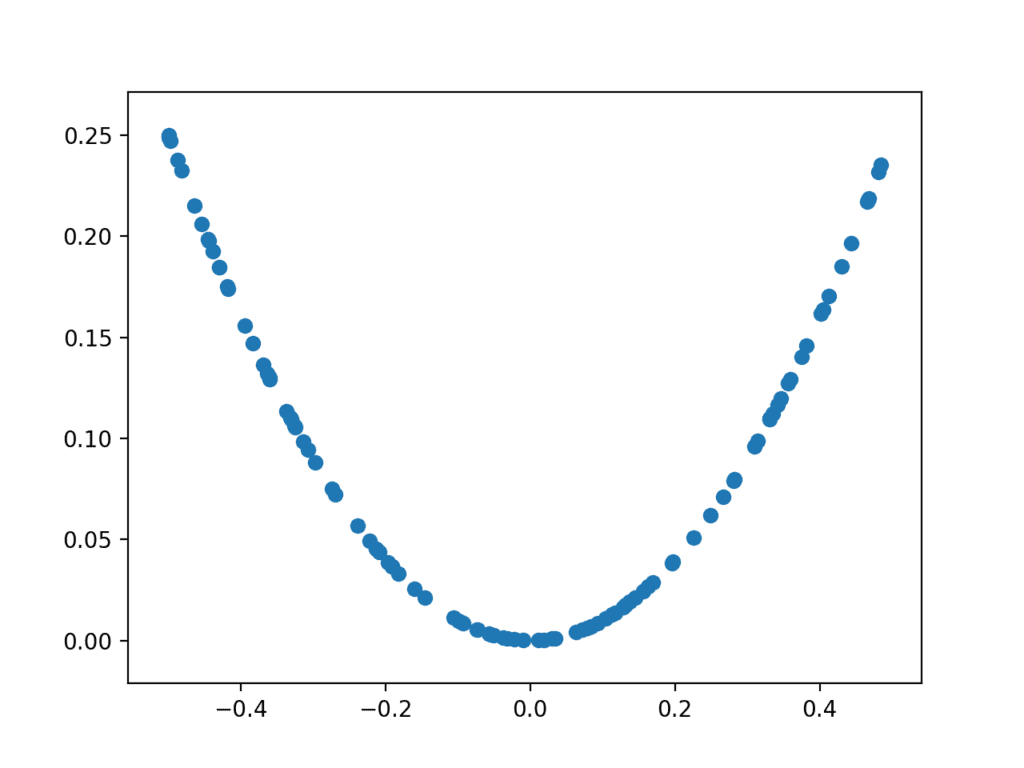
Plot of randomly generated sample of inputs vs. calculated outputs for X^2 function.

We can use this function as a starting point for generating real samples for our discriminator function. Specifically, a sample is comprised of a vector with two elements, one for the input and one for the output of our one-dimensional function.

We can also imagine how a generator model could generate new samples that we can plot and compare to the expected u-shape of the X^2 function. Specifically, a generator would output a vector with two elements: one for the input and one for the output of our one-dimensional function.

Define a Discriminator Model

The next step is to define the discriminator model.

The model must take a sample from our problem, such as a vector with two elements, and output a classification prediction as to whether the sample is real or fake.

This is a binary classification problem.

Inputs: Sample with two real values.
Outputs: Binary classification, likelihood the sample is real (or fake).

The problem is very simple, meaning that we don’t need a complex neural network to model it.

The discriminator model will have one hidden layer with 25 nodes and we will use the ReLU activation function and an appropriate weight initialization method called He weight initialization.

The output layer will have one node for the binary classification using the sigmoid activation function.

The model will minimize the binary cross entropy loss function, and the Adam version of stochastic gradient descent will be used because it is very effective.

The define_discriminator() function below defines and returns the discriminator model. The function parameterizes the number of inputs to expect, which defaults to two.

# define the standalone discriminator model
def define_discriminator(n_inputs=2):
	model = Sequential()
	model.add(Dense(25, activation='relu', kernel_initializer='he_uniform', input_dim=n_inputs))
	model.add(Dense(1, activation='sigmoid'))
	# compile model
	model.compile(loss='binary_crossentropy', optimizer='adam', metrics=['accuracy'])
	return model

We can use this function to define the discriminator model and summarize it. The complete example is listed below.

# define the discriminator model
from keras.models import Sequential
from keras.layers import Dense
from keras.utils.vis_utils import plot_model

# define the standalone discriminator model
def define_discriminator(n_inputs=2):
	model = Sequential()
	model.add(Dense(25, activation='relu', kernel_initializer='he_uniform', input_dim=n_inputs))
	model.add(Dense(1, activation='sigmoid'))
	# compile model
	model.compile(loss='binary_crossentropy', optimizer='adam', metrics=['accuracy'])
	return model

# define the discriminator model
model = define_discriminator()
# summarize the model
model.summary()
# plot the model
plot_model(model, to_file='discriminator_plot.png', show_shapes=True, show_layer_names=True)

Running the example defines the discriminator model and summarizes it.

_________________________________________________________________
Layer (type)                 Output Shape              Param #
=================================================================
dense_1 (Dense)              (None, 25)                75
_________________________________________________________________
dense_2 (Dense)              (None, 1)                 26
=================================================================
Total params: 101
Trainable params: 101
Non-trainable params: 0
_________________________________________________________________

A plot of the model is also created and we can see that the model expects two inputs and will predict a single output.

Note: creating this plot assumes that the pydot and graphviz libraries are installed. If this is a problem, you can comment out the import statement for the plot_model function and the call to the plot_model() function.

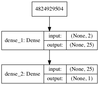
Plot of the Discriminator Model in the GAN

We could start training this model now with real examples with a class label of one and randomly generated samples with a class label of zero.

There is no need to do this, but the elements we will develop will be useful later, and it helps to see that the discriminator is just a normal neural network model.

First, we can update our generate_samples() function from the prediction section and call it generate_real_samples() and have it also return the output class labels for the real samples, specifically, an array of 1 values, where class=1 means real.

# generate n real samples with class labels
def generate_real_samples(n):
	# generate inputs in [-0.5, 0.5]
	X1 = rand(n) - 0.5
	# generate outputs X^2
	X2 = X1 * X1
	# stack arrays
	X1 = X1.reshape(n, 1)
	X2 = X2.reshape(n, 1)
	X = hstack((X1, X2))
	# generate class labels
	y = ones((n, 1))
	return X, y

Next, we can create a copy of this function for creating fake examples.

In this case, we will generate random values in the range -1 and 1 for both elements of a sample. The output class label for all of these examples is 0.

This function will act as our fake generator model.

# generate n fake samples with class labels
def generate_fake_samples(n):
	# generate inputs in [-1, 1]
	X1 = -1 + rand(n) * 2
	# generate outputs in [-1, 1]
	X2 = -1 + rand(n) * 2
	# stack arrays
	X1 = X1.reshape(n, 1)
	X2 = X2.reshape(n, 1)
	X = hstack((X1, X2))
	# generate class labels
	y = zeros((n, 1))
	return X, y

Next, we need a function to train and evaluate the discriminator model.

This can be achieved by manually enumerating the training epochs and for each epoch generating a half batch of real examples and a half batch of fake examples, and updating the model on each, e.g. one whole batch of examples. The train() function could be used, but in this case, we will use the train_on_batch() function directly.

The model can then be evaluated on the generated examples and we can report the classification accuracy on the real and fake samples.

The train_discriminator() function below implements this, training the model for 1,000 batches and using 128 samples per batch (64 fake and 64 real).

# train the discriminator model
def train_discriminator(model, n_epochs=1000, n_batch=128):
	half_batch = int(n_batch / 2)
	# run epochs manually
	for i in range(n_epochs):
		# generate real examples
		X_real, y_real = generate_real_samples(half_batch)
		# update model
		model.train_on_batch(X_real, y_real)
		# generate fake examples
		X_fake, y_fake = generate_fake_samples(half_batch)
		# update model
		model.train_on_batch(X_fake, y_fake)
		# evaluate the model
		_, acc_real = model.evaluate(X_real, y_real, verbose=0)
		_, acc_fake = model.evaluate(X_fake, y_fake, verbose=0)
		print(i, acc_real, acc_fake)

We can tie all of this together and train the discriminator model on real and fake examples.

The complete example is listed below.

# define and fit a discriminator model
from numpy import zeros
from numpy import ones
from numpy import hstack
from numpy.random import rand
from numpy.random import randn
from keras.models import Sequential
from keras.layers import Dense

# define the standalone discriminator model
def define_discriminator(n_inputs=2):
	model = Sequential()
	model.add(Dense(25, activation='relu', kernel_initializer='he_uniform', input_dim=n_inputs))
	model.add(Dense(1, activation='sigmoid'))
	# compile model
	model.compile(loss='binary_crossentropy', optimizer='adam', metrics=['accuracy'])
	return model

# generate n real samples with class labels
def generate_real_samples(n):
	# generate inputs in [-0.5, 0.5]
	X1 = rand(n) - 0.5
	# generate outputs X^2
	X2 = X1 * X1
	# stack arrays
	X1 = X1.reshape(n, 1)
	X2 = X2.reshape(n, 1)
	X = hstack((X1, X2))
	# generate class labels
	y = ones((n, 1))
	return X, y

# generate n fake samples with class labels
def generate_fake_samples(n):
	# generate inputs in [-1, 1]
	X1 = -1 + rand(n) * 2
	# generate outputs in [-1, 1]
	X2 = -1 + rand(n) * 2
	# stack arrays
	X1 = X1.reshape(n, 1)
	X2 = X2.reshape(n, 1)
	X = hstack((X1, X2))
	# generate class labels
	y = zeros((n, 1))
	return X, y

# train the discriminator model
def train_discriminator(model, n_epochs=1000, n_batch=128):
	half_batch = int(n_batch / 2)
	# run epochs manually
	for i in range(n_epochs):
		# generate real examples
		X_real, y_real = generate_real_samples(half_batch)
		# update model
		model.train_on_batch(X_real, y_real)
		# generate fake examples
		X_fake, y_fake = generate_fake_samples(half_batch)
		# update model
		model.train_on_batch(X_fake, y_fake)
		# evaluate the model
		_, acc_real = model.evaluate(X_real, y_real, verbose=0)
		_, acc_fake = model.evaluate(X_fake, y_fake, verbose=0)
		print(i, acc_real, acc_fake)

# define the discriminator model
model = define_discriminator()
# fit the model
train_discriminator(model)

Running the example generates real and fake examples and updates the model, then evaluates the model on the same examples and prints the classification accuracy.

Your specific results may vary but the model rapidly learns to correctly identify the real examples with perfect accuracy and is very good at identifying the fake examples with 80% to 90% accuracy.

...
995 1.0 0.875
996 1.0 0.921875
997 1.0 0.859375
998 1.0 0.9375
999 1.0 0.8125

Training the discriminator model is straightforward. The goal is to train a generator model, not a discriminator model, and that is where the complexity of GANs truly lies.

Define a Generator Model

The next step is to define the generator model.

The generator model takes as input a point from the latent space and generates a new sample, e.g. a vector with both the input and output elements of our function, e.g. x and x^2.

A latent variable is a hidden or unobserved variable, and a latent space is a multi-dimensional vector space of these variables. We can define the size of the latent space for our problem and the shape or distribution of variables in the latent space.

This is because the latent space has no meaning until the generator model starts assigning meaning to points in the space as it learns. After training, points in the latent space will correspond to points in the output space, e.g. in the space of generated samples.

We will define a small latent space of five dimensions and use the standard approach in the GAN literature of using a Gaussian distribution for each variable in the latent space. We will generate new inputs by drawing random numbers from a standard Gaussian distribution, i.e. mean of zero and a standard deviation of one.

Inputs: Point in latent space, e.g. a five-element vector of Gaussian random numbers.
Outputs: Two-element vector representing a generated sample for our function (x and x^2).

The generator model will be small like the discriminator model.

It will have a single hidden layer with five nodes and will use the ReLU activation function and the He weight initialization. The output layer will have two nodes for the two elements in a generated vector and will use a linear activation function.

A linear activation function is used because we know we want the generator to output a vector of real values and the scale will be [-0.5, 0.5] for the first element and about [0.0, 0.25] for the second element.

The model is not compiled. The reason for this is that the generator model is not fit directly.

The define_generator() function below defines and returns the generator model.

The size of the latent dimension is parameterized in case we want to play with it later, and the output shape of the model is also parameterized, matching the function for defining the discriminator model.

# define the standalone generator model
def define_generator(latent_dim, n_outputs=2):
	model = Sequential()
	model.add(Dense(15, activation='relu', kernel_initializer='he_uniform', input_dim=latent_dim))
	model.add(Dense(n_outputs, activation='linear'))
	return model

We can summarize the model to help better understand the input and output shapes.

The complete example is listed below.

# define the generator model
from keras.models import Sequential
from keras.layers import Dense
from keras.utils.vis_utils import plot_model

# define the standalone generator model
def define_generator(latent_dim, n_outputs=2):
	model = Sequential()
	model.add(Dense(15, activation='relu', kernel_initializer='he_uniform', input_dim=latent_dim))
	model.add(Dense(n_outputs, activation='linear'))
	return model

# define the discriminator model
model = define_generator(5)
# summarize the model
model.summary()
# plot the model
plot_model(model, to_file='generator_plot.png', show_shapes=True, show_layer_names=True)

Running the example defines the generator model and summarizes it.

_________________________________________________________________
Layer (type)                 Output Shape              Param #
=================================================================
dense_1 (Dense)              (None, 15)                90
_________________________________________________________________
dense_2 (Dense)              (None, 2)                 32
=================================================================
Total params: 122
Trainable params: 122
Non-trainable params: 0
_________________________________________________________________

A plot of the model is also created and we can see that the model expects a five-element point from the latent space as input and will predict a two-element vector as output.

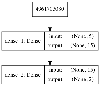
Plot of the Generator Model in the GAN

We can see that the model takes as input a random five-element vector from the latent space and outputs a two-element vector for our one-dimensional function.

This model cannot do much at the moment. Nevertheless, we can demonstrate how to use it to generate samples. This is not needed, but again, some of these elements may be useful later.

The first step is to generate new points in the latent space. We can achieve this by calling the randn() NumPy function for generating arrays of random numbers drawn from a standard Gaussian.

The array of random numbers can then be reshaped into samples: that is n rows with five elements per row. The generate_latent_points() function below implements this and generates the desired number of points in the latent space that can be used as input to the generator model.

# generate points in latent space as input for the generator
def generate_latent_points(latent_dim, n):
	# generate points in the latent space
	x_input = randn(latent_dim * n)
	# reshape into a batch of inputs for the network
	x_input = x_input.reshape(n, latent_dim)
	return x_input

Next, we can use the generated points as input the generator model to generate new samples, then plot the samples.

The generate_fake_samples() function below implements this, where the defined generator and size of the latent space are passed as arguments, along with the number of points for the model to generate.

# use the generator to generate n fake examples and plot the results
def generate_fake_samples(generator, latent_dim, n):
	# generate points in latent space
	x_input = generate_latent_points(latent_dim, n)
	# predict outputs
	X = generator.predict(x_input)
	# plot the results
	pyplot.scatter(X[:, 0], X[:, 1])
	pyplot.show()

Tying this together, the complete example is listed below.

# define and use the generator model
from numpy.random import randn
from keras.models import Sequential
from keras.layers import Dense
from matplotlib import pyplot

# define the standalone generator model
def define_generator(latent_dim, n_outputs=2):
	model = Sequential()
	model.add(Dense(15, activation='relu', kernel_initializer='he_uniform', input_dim=latent_dim))
	model.add(Dense(n_outputs, activation='linear'))
	return model

# generate points in latent space as input for the generator
def generate_latent_points(latent_dim, n):
	# generate points in the latent space
	x_input = randn(latent_dim * n)
	# reshape into a batch of inputs for the network
	x_input = x_input.reshape(n, latent_dim)
	return x_input

# use the generator to generate n fake examples and plot the results
def generate_fake_samples(generator, latent_dim, n):
	# generate points in latent space
	x_input = generate_latent_points(latent_dim, n)
	# predict outputs
	X = generator.predict(x_input)
	# plot the results
	pyplot.scatter(X[:, 0], X[:, 1])
	pyplot.show()

# size of the latent space
latent_dim = 5
# define the discriminator model
model = define_generator(latent_dim)
# generate and plot generated samples
generate_fake_samples(model, latent_dim, 100)

Running the example generates 100 random points from the latent space, uses this as input to the generator and generates 100 fake samples from our one-dimensional function domain.

As the generator has not been trained, the generated points are complete rubbish, as we expect, but we can imagine that as the model is trained, these points will slowly begin to resemble the target function and its u-shape.

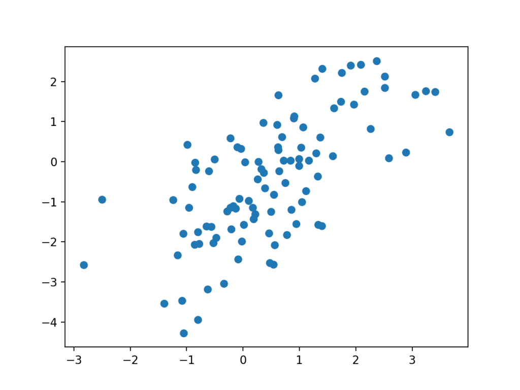
Scatter plot of Fake Samples Predicted by the Generator Model.

We have now seen how to define and use the generator model. We will need to use the generator model in this way to create samples for the discriminator to classify.

We have not seen how the generator model is trained; that is next.

Training the Generator Model

The weights in the generator model are updated based on the performance of the discriminator model.

When the discriminator is good at detecting fake samples, the generator is updated more, and when the discriminator model is relatively poor or confused when detecting fake samples, the generator model is updated less.

This defines the zero-sum or adversarial relationship between these two models.

There may be many ways to implement this using the Keras API, but perhaps the simplest approach is to create a new model that subsumes or encapsulates the generator and discriminator models.

Specifically, a new GAN model can be defined that stacks the generator and discriminator such that the generator receives as input random points in the latent space, generates samples that are fed into the discriminator model directly, classified, and the output of this larger model can be used to update the model weights of the generator.

To be clear, we are not talking about a new third model, just a logical third model that uses the already-defined layers and weights from the standalone generator and discriminator models.

Only the discriminator is concerned with distinguishing between real and fake examples; therefore, the discriminator model can be trained in a standalone manner on examples of each.

The generator model is only concerned with the discriminator’s performance on fake examples. Therefore, we will mark all of the layers in the discriminator as not trainable when it is part of the GAN model so that they can not be updated and overtrained on fake examples.

When training the generator via this subsumed GAN model, there is one more important change. We want the discriminator to think that the samples output by the generator are real, not fake. Therefore, when the generator is trained as part of the GAN model, we will mark the generated samples as real (class 1).

We can imagine that the discriminator will then classify the generated samples as not real (class 0) or a low probability of being real (0.3 or 0.5). The backpropagation process used to update the model weights will see this as a large error and will update the model weights (i.e. only the weights in the generator) to correct for this error, in turn making the generator better at generating plausible fake samples.

Let’s make this concrete.

Inputs: Point in latent space, e.g. a five-element vector of Gaussian random numbers.
Outputs: Binary classification, likelihood the sample is real (or fake).

The define_gan() function below takes as arguments the already-defined generator and discriminator models and creates the new logical third model subsuming these two models. The weights in the discriminator are marked as not trainable, which only affects the weights as seen by the GAN model and not the standalone discriminator model.

The GAN model then uses the same binary cross entropy loss function as the discriminator and the efficient Adam version of stochastic gradient descent.

# define the combined generator and discriminator model, for updating the generator
def define_gan(generator, discriminator):
	# make weights in the discriminator not trainable
	discriminator.trainable = False
	# connect them
	model = Sequential()
	# add generator
	model.add(generator)
	# add the discriminator
	model.add(discriminator)
	# compile model
	model.compile(loss='binary_crossentropy', optimizer='adam')
	return model

Making the discriminator not trainable is a clever trick in the Keras API.

The trainable property impacts the model when it is compiled. The discriminator model was compiled with trainable layers, therefore the model weights in those layers will be updated when the standalone model is updated via calls to train_on_batch().

The discriminator model was marked as not trainable, added to the GAN model, and compiled. In this model, the model weights of the discriminator model are not trainable and cannot be changed when the GAN model is updated via calls to train_on_batch().

This behavior is described in the Keras API documentation here:

How can I “freeze” Keras layers?

The complete example of creating the discriminator, generator, and composite model is listed below.

# demonstrate creating the three models in the gan
from keras.models import Sequential
from keras.layers import Dense
from keras.utils.vis_utils import plot_model

# define the standalone discriminator model
def define_discriminator(n_inputs=2):
	model = Sequential()
	model.add(Dense(25, activation='relu', kernel_initializer='he_uniform', input_dim=n_inputs))
	model.add(Dense(1, activation='sigmoid'))
	# compile model
	model.compile(loss='binary_crossentropy', optimizer='adam', metrics=['accuracy'])
	return model

# define the standalone generator model
def define_generator(latent_dim, n_outputs=2):
	model = Sequential()
	model.add(Dense(15, activation='relu', kernel_initializer='he_uniform', input_dim=latent_dim))
	model.add(Dense(n_outputs, activation='linear'))
	return model

# define the combined generator and discriminator model, for updating the generator
def define_gan(generator, discriminator):
	# make weights in the discriminator not trainable
	discriminator.trainable = False
	# connect them
	model = Sequential()
	# add generator
	model.add(generator)
	# add the discriminator
	model.add(discriminator)
	# compile model
	model.compile(loss='binary_crossentropy', optimizer='adam')
	return model

# size of the latent space
latent_dim = 5
# create the discriminator
discriminator = define_discriminator()
# create the generator
generator = define_generator(latent_dim)
# create the gan
gan_model = define_gan(generator, discriminator)
# summarize gan model
gan_model.summary()
# plot gan model
plot_model(gan_model, to_file='gan_plot.png', show_shapes=True, show_layer_names=True)

Running the example first creates a summary of the composite model.

_________________________________________________________________
Layer (type)                 Output Shape              Param #
=================================================================
sequential_2 (Sequential)    (None, 2)                 122
_________________________________________________________________
sequential_1 (Sequential)    (None, 1)                 101
=================================================================
Total params: 223
Trainable params: 122
Non-trainable params: 101
_________________________________________________________________

A plot of the model is also created and we can see that the model expects a five-element point in latent space as input and will predict a single output classification label.

Note, creating this plot assumes that the pydot and graphviz libraries are installed. If this is a problem, you can comment out the import statement for the plot_model function and the call to the plot_model() function.

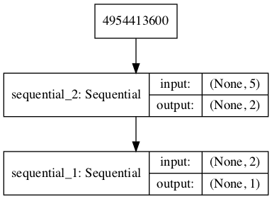
Plot of the Composite Generator and Discriminator Model in the GAN

Training the composite model involves generating a batch-worth of points in the latent space via the generate_latent_points() function in the previous section, and class=1 labels and calling the train_on_batch() function.

The train_gan() function below demonstrates this, although it is pretty uninteresting as only the generator will be updated each epoch, leaving the discriminator with default model weights.

# train the composite model
def train_gan(gan_model, latent_dim, n_epochs=10000, n_batch=128):
	# manually enumerate epochs
	for i in range(n_epochs):
		# prepare points in latent space as input for the generator
		x_gan = generate_latent_points(latent_dim, n_batch)
		# create inverted labels for the fake samples
		y_gan = ones((n_batch, 1))
		# update the generator via the discriminator's error
		gan_model.train_on_batch(x_gan, y_gan)

Instead, what is required is that we first update the discriminator model with real and fake samples, then update the generator via the composite model.

This requires combining elements from the train_discriminator() function defined in the discriminator section and the train_gan() function defined above. It also requires that the generate_fake_samples() function use the generator model to generate fake samples instead of generating random numbers.

The complete train function for updating the discriminator model and the generator (via the composite model) is listed below.

# train the generator and discriminator
def train(g_model, d_model, gan_model, latent_dim, n_epochs=10000, n_batch=128):
	# determine half the size of one batch, for updating the discriminator
	half_batch = int(n_batch / 2)
	# manually enumerate epochs
	for i in range(n_epochs):
		# prepare real samples
		x_real, y_real = generate_real_samples(half_batch)
		# prepare fake examples
		x_fake, y_fake = generate_fake_samples(g_model, latent_dim, half_batch)
		# update discriminator
		d_model.train_on_batch(x_real, y_real)
		d_model.train_on_batch(x_fake, y_fake)
		# prepare points in latent space as input for the generator
		x_gan = generate_latent_points(latent_dim, n_batch)
		# create inverted labels for the fake samples
		y_gan = ones((n_batch, 1))
		# update the generator via the discriminator's error
		gan_model.train_on_batch(x_gan, y_gan)

We almost have everything we need to develop a GAN for our one-dimensional function.

One remaining aspect is the evaluation of the model.

Evaluating the Performance of the GAN

Generally, there are no objective ways to evaluate the performance of a GAN model.

In this specific case, we can devise an objective measure for the generated samples as we know the true underlying input domain and target function and can calculate an objective error measure.

Nevertheless, we will not calculate this objective error score in this tutorial. Instead, we will use the subjective approach used in most GAN applications. Specifically, we will use the generator to generate new samples and inspect them relative to real samples from the domain.

First, we can use the generate_real_samples() function developed in the discriminator part above to generate real examples. Creating a scatter plot of these examples will create the familiar u-shape of our target function.

# generate n real samples with class labels
def generate_real_samples(n):
	# generate inputs in [-0.5, 0.5]
	X1 = rand(n) - 0.5
	# generate outputs X^2
	X2 = X1 * X1
	# stack arrays
	X1 = X1.reshape(n, 1)
	X2 = X2.reshape(n, 1)
	X = hstack((X1, X2))
	# generate class labels
	y = ones((n, 1))
	return X, y

Next, we can use the generator model to generate the same number of fake samples.

This requires first generating the same number of points in the latent space via the generate_latent_points() function developed in the generator section above. These can then be passed to the generator model and used to generate samples that can also be plotted on the same scatter plot.

# generate points in latent space as input for the generator
def generate_latent_points(latent_dim, n):
	# generate points in the latent space
	x_input = randn(latent_dim * n)
	# reshape into a batch of inputs for the network
	x_input = x_input.reshape(n, latent_dim)
	return x_input

The generate_fake_samples() function below generates these fake samples and the associated class label of 0 which will be useful later.

# use the generator to generate n fake examples, with class labels
def generate_fake_samples(generator, latent_dim, n):
	# generate points in latent space
	x_input = generate_latent_points(latent_dim, n)
	# predict outputs
	X = generator.predict(x_input)
	# create class labels
	y = zeros((n, 1))
	return X, y

Having both samples plotted on the same graph allows them to be directly compared to see if the same input and output domain are covered and whether the expected shape of the target function has been appropriately captured, at least subjectively.

The summarize_performance() function below can be called any time during training to create a scatter plot of real and generated points to get an idea of the current capability of the generator model.

# plot real and fake points
def summarize_performance(generator, latent_dim, n=100):
	# prepare real samples
	x_real, y_real = generate_real_samples(n)
	# prepare fake examples
	x_fake, y_fake = generate_fake_samples(generator, latent_dim, n)
	# scatter plot real and fake data points
	pyplot.scatter(x_real[:, 0], x_real[:, 1], color='red')
	pyplot.scatter(x_fake[:, 0], x_fake[:, 1], color='blue')
	pyplot.show()

We may also be interested in the performance of the discriminator model at the same time.

Specifically, we are interested to know how well the discriminator model can correctly identify real and fake samples. A good generator model should make the discriminator model confused, resulting in a classification accuracy closer to 50% on real and fake examples.

We can update the summarize_performance() function to also take the discriminator and current epoch number as arguments and report the accuracy on the sample of real and fake examples.

# evaluate the discriminator and plot real and fake points
def summarize_performance(epoch, generator, discriminator, latent_dim, n=100):
	# prepare real samples
	x_real, y_real = generate_real_samples(n)
	# evaluate discriminator on real examples
	_, acc_real = discriminator.evaluate(x_real, y_real, verbose=0)
	# prepare fake examples
	x_fake, y_fake = generate_fake_samples(generator, latent_dim, n)
	# evaluate discriminator on fake examples
	_, acc_fake = discriminator.evaluate(x_fake, y_fake, verbose=0)
	# summarize discriminator performance
	print(epoch, acc_real, acc_fake)
	# scatter plot real and fake data points
	pyplot.scatter(x_real[:, 0], x_real[:, 1], color='red')
	pyplot.scatter(x_fake[:, 0], x_fake[:, 1], color='blue')
	pyplot.show()

This function can then be called periodically during training.

For example, if we choose to train the models for 10,000 iterations, it may be interesting to check-in on the performance of the model every 2,000 iterations.

We can achieve this by parameterizing the frequency of the check-in via n_eval argument, and calling the summarize_performance() function from the train() function after the appropriate number of iterations.

The updated version of the train() function with this change is listed below.

# train the generator and discriminator
def train(g_model, d_model, gan_model, latent_dim, n_epochs=10000, n_batch=128, n_eval=2000):
	# determine half the size of one batch, for updating the discriminator
	half_batch = int(n_batch / 2)
	# manually enumerate epochs
	for i in range(n_epochs):
		# prepare real samples
		x_real, y_real = generate_real_samples(half_batch)
		# prepare fake examples
		x_fake, y_fake = generate_fake_samples(g_model, latent_dim, half_batch)
		# update discriminator
		d_model.train_on_batch(x_real, y_real)
		d_model.train_on_batch(x_fake, y_fake)
		# prepare points in latent space as input for the generator
		x_gan = generate_latent_points(latent_dim, n_batch)
		# create inverted labels for the fake samples
		y_gan = ones((n_batch, 1))
		# update the generator via the discriminator's error
		gan_model.train_on_batch(x_gan, y_gan)
		# evaluate the model every n_eval epochs
		if (i+1) % n_eval == 0:
			summarize_performance(i, g_model, d_model, latent_dim)

Complete Example of Training the GAN

We now have everything we need to train and evaluate a GAN on our chosen one-dimensional function.

The complete example is listed below.

# train a generative adversarial network on a one-dimensional function
from numpy import hstack
from numpy import zeros
from numpy import ones
from numpy.random import rand
from numpy.random import randn
from keras.models import Sequential
from keras.layers import Dense
from matplotlib import pyplot

# define the standalone discriminator model
def define_discriminator(n_inputs=2):
	model = Sequential()
	model.add(Dense(25, activation='relu', kernel_initializer='he_uniform', input_dim=n_inputs))
	model.add(Dense(1, activation='sigmoid'))
	# compile model
	model.compile(loss='binary_crossentropy', optimizer='adam', metrics=['accuracy'])
	return model

# define the standalone generator model
def define_generator(latent_dim, n_outputs=2):
	model = Sequential()
	model.add(Dense(15, activation='relu', kernel_initializer='he_uniform', input_dim=latent_dim))
	model.add(Dense(n_outputs, activation='linear'))
	return model

# define the combined generator and discriminator model, for updating the generator
def define_gan(generator, discriminator):
	# make weights in the discriminator not trainable
	discriminator.trainable = False
	# connect them
	model = Sequential()
	# add generator
	model.add(generator)
	# add the discriminator
	model.add(discriminator)
	# compile model
	model.compile(loss='binary_crossentropy', optimizer='adam')
	return model

# generate n real samples with class labels
def generate_real_samples(n):
	# generate inputs in [-0.5, 0.5]
	X1 = rand(n) - 0.5
	# generate outputs X^2
	X2 = X1 * X1
	# stack arrays
	X1 = X1.reshape(n, 1)
	X2 = X2.reshape(n, 1)
	X = hstack((X1, X2))
	# generate class labels
	y = ones((n, 1))
	return X, y

# generate points in latent space as input for the generator
def generate_latent_points(latent_dim, n):
	# generate points in the latent space
	x_input = randn(latent_dim * n)
	# reshape into a batch of inputs for the network
	x_input = x_input.reshape(n, latent_dim)
	return x_input

# use the generator to generate n fake examples, with class labels
def generate_fake_samples(generator, latent_dim, n):
	# generate points in latent space
	x_input = generate_latent_points(latent_dim, n)
	# predict outputs
	X = generator.predict(x_input)
	# create class labels
	y = zeros((n, 1))
	return X, y

# evaluate the discriminator and plot real and fake points
def summarize_performance(epoch, generator, discriminator, latent_dim, n=100):
	# prepare real samples
	x_real, y_real = generate_real_samples(n)
	# evaluate discriminator on real examples
	_, acc_real = discriminator.evaluate(x_real, y_real, verbose=0)
	# prepare fake examples
	x_fake, y_fake = generate_fake_samples(generator, latent_dim, n)
	# evaluate discriminator on fake examples
	_, acc_fake = discriminator.evaluate(x_fake, y_fake, verbose=0)
	# summarize discriminator performance
	print(epoch, acc_real, acc_fake)
	# scatter plot real and fake data points
	pyplot.scatter(x_real[:, 0], x_real[:, 1], color='red')
	pyplot.scatter(x_fake[:, 0], x_fake[:, 1], color='blue')
	pyplot.show()

# train the generator and discriminator
def train(g_model, d_model, gan_model, latent_dim, n_epochs=10000, n_batch=128, n_eval=2000):
	# determine half the size of one batch, for updating the discriminator
	half_batch = int(n_batch / 2)
	# manually enumerate epochs
	for i in range(n_epochs):
		# prepare real samples
		x_real, y_real = generate_real_samples(half_batch)
		# prepare fake examples
		x_fake, y_fake = generate_fake_samples(g_model, latent_dim, half_batch)
		# update discriminator
		d_model.train_on_batch(x_real, y_real)
		d_model.train_on_batch(x_fake, y_fake)
		# prepare points in latent space as input for the generator
		x_gan = generate_latent_points(latent_dim, n_batch)
		# create inverted labels for the fake samples
		y_gan = ones((n_batch, 1))
		# update the generator via the discriminator's error
		gan_model.train_on_batch(x_gan, y_gan)
		# evaluate the model every n_eval epochs
		if (i+1) % n_eval == 0:
			summarize_performance(i, g_model, d_model, latent_dim)

# size of the latent space
latent_dim = 5
# create the discriminator
discriminator = define_discriminator()
# create the generator
generator = define_generator(latent_dim)
# create the gan
gan_model = define_gan(generator, discriminator)
# train model
train(generator, discriminator, gan_model, latent_dim)

Running the example reports model performance every 2,000 training iterations (batches) and creates a plot.

Your specific results may vary given the stochastic nature of the training algorithm, and the generative model itself.

We can see that the training process is relatively unstable. The first column reports the iteration number, the second the classification accuracy of the discriminator for real examples, and the third column the classification accuracy of the discriminator for generated (fake) examples.

In this case, we can see that the discriminator remains relatively confused about real examples, and performance on identifying fake examples varies.

1999 0.45 1.0
3999 0.45 0.91
5999 0.86 0.16
7999 0.6 0.41
9999 0.15 0.93

I will omit providing the five created plots here for brevity; instead we will look at only two.

The first plot is created after 2,000 iterations and shows real (red) vs. fake (blue) samples. The model performs poorly initially with a cluster of generated points only in the positive input domain, although with the right functional relationship.

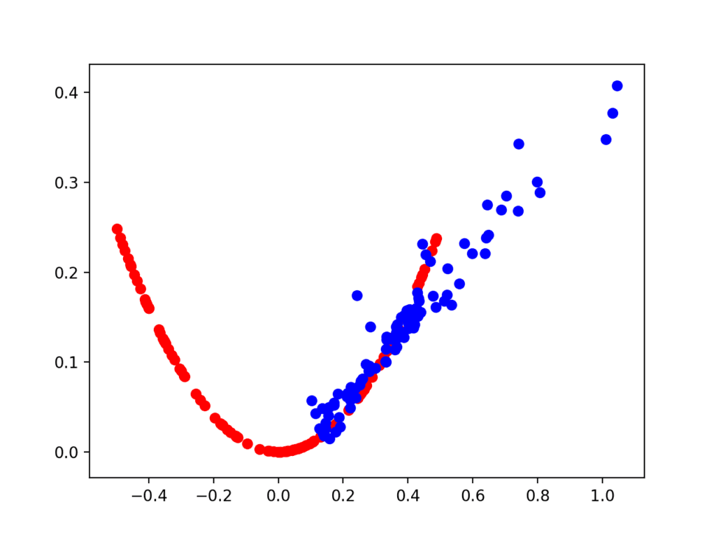
Scatter Plot of Real and Generated Examples for the Target Function After 2,000 Iterations.

The second plot shows real (red) vs. fake (blue) after 10,000 iterations.

Here we can see that the generator model does a reasonable job of generating plausible samples, with the input values in the right domain between [-0.5 and 0.5] and the output values showing the X^2 relationship, or close to it.

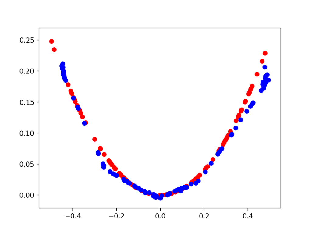
Scatter Plot of Real and Generated Examples for the Target Function After 10,000 Iterations.

Extensions

This section lists some ideas for extending the tutorial that you may wish to explore.

Model Architecture. Experiment with alternate model architectures for the discriminator and generator, such as more or fewer nodes, layers, and alternate activation functions such as leaky ReLU.
Data Scaling. Experiment with alternate activation functions such as the hyperbolic tangent (tanh) and any required scaling of training data.
Alternate Target Function. Experiment with an alternate target function, such a simple sine wave, Gaussian distribution, a different quadratic, or even a multi-modal polynomial function.

If you explore any of these extensions, I’d love to know.
Post your findings in the comments below.

Summary

In this tutorial, you discovered how to develop a generative adversarial network from scratch for a one-dimensional function.

Specifically, you learned:

The benefit of developing a generative adversarial network from scratch for a simple one-dimensional function.
How to develop separate discriminator and generator models, as well as a composite model for training the generator via the discriminator’s predictive behavior.
How to subjectively evaluate generated samples in the context of real examples from the problem domain.

Do you have any questions?
Ask your questions in the comments below and I will do my best to answer.

The post How to Develop a 1D Generative Adversarial Network From Scratch in Keras appeared first on Machine Learning Mastery.

Go to Source

Tutorial Overview

Select a One-Dimensional Function

Define a Discriminator Model

Define a Generator Model

Training the Generator Model

Evaluating the Performance of the GAN

Complete Example of Training the GAN

Extensions

Further Reading

API

Summary