Author: Jason Brownlee
Generative Adversarial Networks, or GANs, are an architecture for training generative models, such as deep convolutional neural networks for generating images.
The generative model in the GAN architecture learns to map points in the latent space to generated images. The latent space has no meaning other than the meaning applied to it via the generative model. Yet, the latent space has structure that can be explored, such as by interpolating between points and performing vector arithmetic between points in latent space which have meaningful and targeted effects on the generated images.
In this tutorial, you will discover how to develop a generative adversarial network for face generation and explore the structure of latent space and the effect on generated faces.
After completing this tutorial, you will know:
- How to develop a generative adversarial network for generating faces.
- How to interpolate between points in latent space and generate images that morph from one face to another.
- How to perform vector arithmetic in latent space and achieve targeted results in the resulting generated faces.
Let’s get started.
How to Interpolate and Perform Vector Arithmetic With Faces Using a Generative Adversarial Network.
Photo by Intermountain Forest Service, some rights reserved.
Tutorial Overview
This tutorial is divided into five parts; they are:
- Vector Arithmetic in Latent Space
- Large-Scale CelebFaces Dataset (CelebA)
- How to Prepare CelebA Faces Dataset
- How to Develop a Generative Adversarial Network
- How to Explore the Latent Space for Generated Faces
Vector Arithmetic in Latent Space
The generator model in the GAN architecture takes a point from the latent space as input and generates a new image.
The latent space itself has no meaning. Typically it is a 100-dimensional hypersphere with each variable drawn from a Gaussian distribution with a mean of zero and a standard deviation of one. Through training, the generator learns to map points into the latent space with specific output images and this mapping will be different each time the model is trained.
The latent space has structure when interpreted by the generator model, and this structure can be queried and navigated for a given model.
Typically, new images are generated using random points in the latent space. Taken a step further, points in the latent space can be constructed (e.g. all 0s, all 0.5s, or all 1s) and used as input or a query to generate a specific image.
A series of points can be created on a linear path between two points in the latent space, such as two generated images. These points can be used to generate a series of images that show a transition between the two generated images.
Finally, the points in the latent space can be kept and used in simple vector arithmetic to create new points in the latent space that, in turn, can be used to generate images. This is an interesting idea, as it allows for the intuitive and targeted generation of images.
The important 2015 paper by Alec Radford, et al. titled “Unsupervised Representation Learning with Deep Convolutional Generative Adversarial Networks” introduced a stable model configuration for training deep convolutional neural network models as part of the GAN architecture.
In the paper, the authors explored the latent space for GANs fit on a number of different training datasets, most notably a dataset of celebrity faces. They demonstrated two interesting aspects.
The first was the vector arithmetic with faces. For example, a face of a smiling woman minus the face of a neutral woman plus the face of a neutral man resulted in the face of a smiling man.
smiling woman - neutral woman + neutral man = smiling man
Specifically, the arithmetic was performed on the points in the latent space for the resulting faces. Actually on the average of multiple faces with a given characteristic, to provide a more robust result.
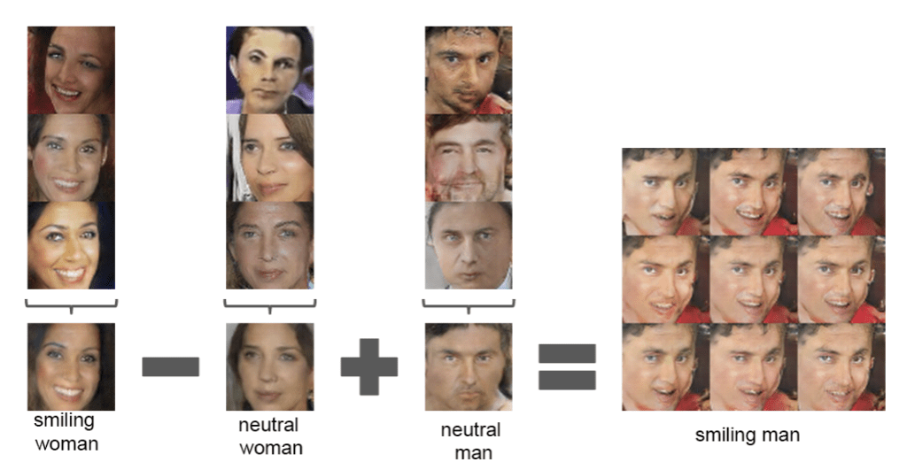
Example of Vector Arithmetic on Points in the Latent Space for Generating Faces With a GAN.
Taken from Unsupervised Representation Learning with Deep Convolutional Generative Adversarial Networks.
The second demonstration was the transition between two generated faces, specifically by creating a linear path through the latent dimension between the points that generated two faces and then generating all of the faces for the points along the path.
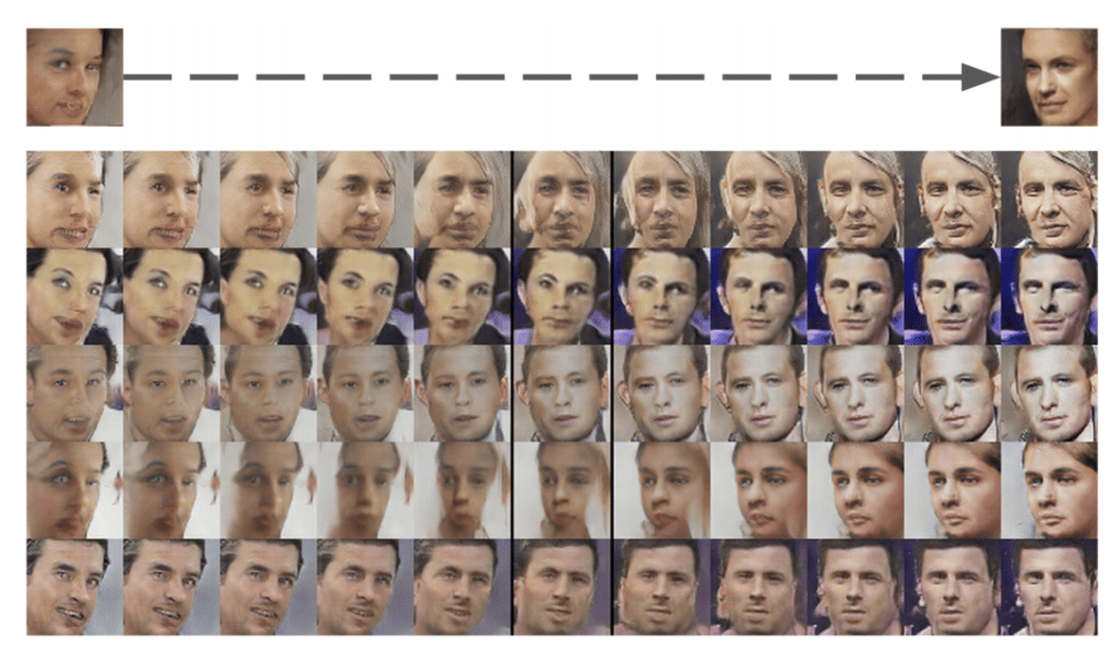
Example of Faces on a Path Between Two GAN Generated Faces.
Taken from Unsupervised Representation Learning with Deep Convolutional Generative Adversarial Networks.
Exploring the structure of the latent space for a GAN model is both interesting for the problem domain and helps to develop an intuition for what has been learned by the generator model.
In this tutorial, we will develop a GAN for generating photos of faces, then explore the latent space for the model with vector arithmetic.
Large-Scale CelebFaces Dataset (CelebA)
The first step is to select a dataset of faces.
In this tutorial, we will use the Large-scale CelebFaces Attributes Dataset, referred to as CelebA. This dataset was developed and published by Ziwei Liu, et al. for their 2015 paper titled “From Facial Parts Responses to Face Detection: A Deep Learning Approach.”
The dataset provides about 200,000 photographs of celebrity faces along with annotations for what appears in given photos, such as glasses, face shape, hats, hair type, etc. As part of the dataset, the authors provide a version of each photo centered on the face and cropped to the portrait with varying sizes around 150 pixels wide and 200 pixels tall. We will use this as the basis for developing our GAN model.
The dataset can be easily downloaded from the Kaggle webpage. Note: this may require an account with Kaggle.
Specifically, download the file “img_align_celeba.zip” which is about 1.3 gigabytes. To do this, click on the filename on the Kaggle website and then click the download icon.
The download might take a while depending on the speed of your internet connection.
After downloading, unzip the archive.
This will create a new directory named “img_align_celeba” that contains all of the images with filenames like 202599.jpg and 202598.jpg.
Next, we can look at preparing the raw images for modeling.
How to Prepare CelebA Faces Dataset
The first step is to develop code to load the images.
We can use the Pillow library to load a given image file, convert it to RGB format (if needed) and return an array of pixel data. The load_image() function below implements this.
# load an image as an rgb numpy array
def load_image(filename):
	# load image from file
	image = Image.open(filename)
	# convert to RGB, if needed
	image = image.convert('RGB')
	# convert to array
	pixels = asarray(image)
	return pixels
Next, we can enumerate the directory of images, load each as an array of pixels in turn, and return an array with all of the images.
There are 200K images in the dataset, which is probably more than we need so we can also limit the number of images to load with an argument. The load_faces() function below implements this.
# load images and extract faces for all images in a directory
def load_faces(directory, n_faces):
	faces = list()
	# enumerate files
	for filename in listdir(directory):
		# load the image
		pixels = load_image(directory + filename)
		# store
		faces.append(pixels)
		# stop once we have enough
		if len(faces) >= n_faces:
			break
	return asarray(faces)
Finally, once the images are loaded, we can plot them using the imshow() function from the matplotlib library.
The plot_faces() function below does this, plotting images arranged into in a square.
# plot a list of loaded faces
def plot_faces(faces, n):
	for i in range(n * n):
		# define subplot
		pyplot.subplot(n, n, 1 + i)
		# turn off axis
		pyplot.axis('off')
		# plot raw pixel data
		pyplot.imshow(faces[i])
	pyplot.show()
Tying this together, the complete example is listed below.
# load and plot faces
from os import listdir
from numpy import asarray
from PIL import Image
from matplotlib import pyplot

# load an image as an rgb numpy array
def load_image(filename):
	# load image from file
	image = Image.open(filename)
	# convert to RGB, if needed
	image = image.convert('RGB')
	# convert to array
	pixels = asarray(image)
	return pixels

# load images and extract faces for all images in a directory
def load_faces(directory, n_faces):
	faces = list()
	# enumerate files
	for filename in listdir(directory):
		# load the image
		pixels = load_image(directory + filename)
		# store
		faces.append(pixels)
		# stop once we have enough
		if len(faces) >= n_faces:
			break
	return asarray(faces)

# plot a list of loaded faces
def plot_faces(faces, n):
	for i in range(n * n):
		# define subplot
		pyplot.subplot(n, n, 1 + i)
		# turn off axis
		pyplot.axis('off')
		# plot raw pixel data
		pyplot.imshow(faces[i])
	pyplot.show()

# directory that contains all images
directory = 'img_align_celeba/'
# load and extract all faces
faces = load_faces(directory, 25)
print('Loaded: ', faces.shape)
# plot faces
plot_faces(faces, 5)
Running the example loads a total of 25 images from the directory, then summarizes the size of the returned array.
Loaded: (25, 218, 178, 3)
Finally, the 25 images are plotted in a 5×5 square.
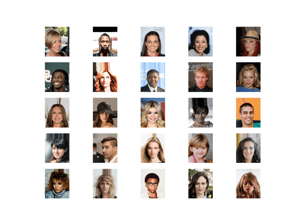
Plot of a Sample of 25 Faces from the Celebrity Faces Dataset
When working with a GAN, it is easier to model a dataset if all of the images are small and square in shape.
Further, as we are only interested in the face in each photo, and not the background, we can perform face detection and extract only the face before resizing the result to a fixed size.
There are many ways to perform face detection. In this case, we will use a pre-trained Multi-Task Cascaded Convolutional Neural Network, or MTCNN. This is a state-of-the-art deep learning model for face detection, described in the 2016 paper titled “Joint Face Detection and Alignment Using Multitask Cascaded Convolutional Networks.”
We will use the implementation provided by Iván de Paz Centeno in the ipazc/mtcnn project. This library can be installed via pip as follows:
sudo pip install mtcnn
We can confirm that the library was installed correctly by importing the library and printing the version; for example:
# confirm mtcnn was installed correctly
import mtcnn
# print version
print(mtcnn.__version__)
Running the example prints the current version of the library.
0.0.8
The MTCNN model is very easy to use.
First, an instance of the MTCNN model is created, then the detect_faces() function can be called passing in the pixel data for one image. The result is a list of detected faces, with a bounding box defined in pixel offset values.
...
# prepare model
model = MTCNN()
# detect face in the image
faces = model.detect_faces(pixels)
# extract details of the face
x1, y1, width, height = faces[0]['box']
We can update our example to extract the face from each loaded photo and resize the extracted face pixels to a fixed size. In this case, we will use the square shape of 80×80 pixels.
The extract_face() function below implements this, taking the MTCNN model and pixel values for a single photograph as arguments and returning an 80x80x3 array of pixel values with just the face, or None if no face was detected (which can happen rarely).
# extract the face from a loaded image and resize
def extract_face(model, pixels, required_size=(80, 80)):
	# detect face in the image
	faces = model.detect_faces(pixels)
	# skip cases where we could not detect a face
	if len(faces) == 0:
		return None
	# extract details of the face
	x1, y1, width, height = faces[0]['box']
	# force detected pixel values to be positive (bug fix)
	x1, y1 = abs(x1), abs(y1)
	# convert into coordinates
	x2, y2 = x1 + width, y1 + height
	# retrieve face pixels
	face_pixels = pixels[y1:y2, x1:x2]
	# resize pixels to the model size
	image = Image.fromarray(face_pixels)
	image = image.resize(required_size)
	face_array = asarray(image)
	return face_array
We can now update the load_faces() function to extract the face from the loaded photo and store that in the list of faces returned.
# load images and extract faces for all images in a directory
def load_faces(directory, n_faces):
	# prepare model
	model = MTCNN()
	faces = list()
	# enumerate files
	for filename in listdir(directory):
		# load the image
		pixels = load_image(directory + filename)
		# get face
		face = extract_face(model, pixels)
		if face is None:
			continue
		# store
		faces.append(face)
		print(len(faces), face.shape)
		# stop once we have enough
		if len(faces) >= n_faces:
			break
	return asarray(faces)
Tying this together, the complete example is listed below.
In this case, we increase the total number of loaded faces to 50,000 to provide a good training dataset for our GAN model.
# example of extracting and resizing faces into a new dataset
from os import listdir
from numpy import asarray
from numpy import savez_compressed
from PIL import Image
from mtcnn.mtcnn import MTCNN
from matplotlib import pyplot

# load an image as an rgb numpy array
def load_image(filename):
	# load image from file
	image = Image.open(filename)
	# convert to RGB, if needed
	image = image.convert('RGB')
	# convert to array
	pixels = asarray(image)
	return pixels

# extract the face from a loaded image and resize
def extract_face(model, pixels, required_size=(80, 80)):
	# detect face in the image
	faces = model.detect_faces(pixels)
	# skip cases where we could not detect a face
	if len(faces) == 0:
		return None
	# extract details of the face
	x1, y1, width, height = faces[0]['box']
	# force detected pixel values to be positive (bug fix)
	x1, y1 = abs(x1), abs(y1)
	# convert into coordinates
	x2, y2 = x1 + width, y1 + height
	# retrieve face pixels
	face_pixels = pixels[y1:y2, x1:x2]
	# resize pixels to the model size
	image = Image.fromarray(face_pixels)
	image = image.resize(required_size)
	face_array = asarray(image)
	return face_array

# load images and extract faces for all images in a directory
def load_faces(directory, n_faces):
	# prepare model
	model = MTCNN()
	faces = list()
	# enumerate files
	for filename in listdir(directory):
		# load the image
		pixels = load_image(directory + filename)
		# get face
		face = extract_face(model, pixels)
		if face is None:
			continue
		# store
		faces.append(face)
		print(len(faces), face.shape)
		# stop once we have enough
		if len(faces) >= n_faces:
			break
	return asarray(faces)

# directory that contains all images
directory = 'img_align_celeba/'
# load and extract all faces
all_faces = load_faces(directory, 50000)
print('Loaded: ', all_faces.shape)
# save in compressed format
savez_compressed('img_align_celeba.npz', all_faces)
Running the example may take a few minutes given the larger number of faces to be loaded.
At the end of the run, the array of extracted and resized faces is saved as a compressed NumPy array with the filename ‘img_align_celeba.npz‘.
The prepared dataset can then be loaded any time, as follows.
# load the prepared dataset
from numpy import load
# load the face dataset
data = load('img_align_celeba.npz')
faces = data['arr_0']
print('Loaded: ', faces.shape)
Loading the dataset summarizes the shape of the array, showing 50K images with the size of 80×80 pixels and three color channels.
Loaded: (50000, 80, 80, 3)
We are now ready to develop a GAN model to generate faces using this dataset.
How to Develop a Generative Adversarial Network
In this section, we will develop a GAN for the faces dataset that we have prepared.
The first step is to define the models.
The discriminator model takes as input one 80×80 color image an outputs a binary prediction as to whether the image is real (class=1) or fake (class=0). It is implemented as a modest convolutional neural network using best practices for GAN design such as using the LeakyReLU activation function with a slope of 0.2, using a 2×2 stride to downsample, and the adam version of stochastic gradient descent with a learning rate of 0.0002 and a momentum of 0.5
The define_discriminator() function below implements this, defining and compiling the discriminator model and returning it. The input shape of the image is parameterized as a default function argument in case you want to re-use the function for your own image data later.
# define the standalone discriminator model
def define_discriminator(in_shape=(80,80,3)):
	model = Sequential()
	# normal
	model.add(Conv2D(128, (5,5), padding='same', input_shape=in_shape))
	model.add(LeakyReLU(alpha=0.2))
	# downsample to 40x40
	model.add(Conv2D(128, (5,5), strides=(2,2), padding='same'))
	model.add(LeakyReLU(alpha=0.2))
	# downsample to 20x30
	model.add(Conv2D(128, (5,5), strides=(2,2), padding='same'))
	model.add(LeakyReLU(alpha=0.2))
	# downsample to 10x10
	model.add(Conv2D(128, (5,5), strides=(2,2), padding='same'))
	model.add(LeakyReLU(alpha=0.2))
	# downsample to 5x5
	model.add(Conv2D(128, (5,5), strides=(2,2), padding='same'))
	model.add(LeakyReLU(alpha=0.2))
	# classifier
	model.add(Flatten())
	model.add(Dropout(0.4))
	model.add(Dense(1, activation='sigmoid'))
	# compile model
	opt = Adam(lr=0.0002, beta_1=0.5)
	model.compile(loss='binary_crossentropy', optimizer=opt, metrics=['accuracy'])
	return model
The generator model takes as input a point in the latent space and outputs a single 80×80 color image.
This is achieved by using a fully connected layer to interpret the point in the latent space and provide sufficient activations that can be reshaped into many copies (in this case 128) of a low-resolution version of the output image (e.g. 5×5). This is then upsampled four times, doubling the size and quadrupling the area of the activations each time using transpose convolutional layers. The model uses best practices such as the LeakyReLU activation, a kernel size that is a factor of the stride size, and a hyperbolic tangent (tanh) activation function in the output layer.
The define_generator() function below defines the generator model but intentionally does not compile it as it is not trained directly, then returns the model. The size of the latent space is parameterized as a function argument.
# define the standalone generator model
def define_generator(latent_dim):
	model = Sequential()
	# foundation for 5x5 feature maps
	n_nodes = 128 * 5 * 5
	model.add(Dense(n_nodes, input_dim=latent_dim))
	model.add(LeakyReLU(alpha=0.2))
	model.add(Reshape((5, 5, 128)))
	# upsample to 10x10
	model.add(Conv2DTranspose(128, (4,4), strides=(2,2), padding='same'))
	model.add(LeakyReLU(alpha=0.2))
	# upsample to 20x20
	model.add(Conv2DTranspose(128, (4,4), strides=(2,2), padding='same'))
	model.add(LeakyReLU(alpha=0.2))
	# upsample to 40x40
	model.add(Conv2DTranspose(128, (4,4), strides=(2,2), padding='same'))
	model.add(LeakyReLU(alpha=0.2))
	# upsample to 80x80
	model.add(Conv2DTranspose(128, (4,4), strides=(2,2), padding='same'))
	model.add(LeakyReLU(alpha=0.2))
	# output layer 80x80x3
	model.add(Conv2D(3, (5,5), activation='tanh', padding='same'))
	return model
Next, a GAN model can be defined that combines both the generator model and the discriminator model into one larger model. This larger model will be used to train the model weights in the generator, using the output and error calculated by the discriminator model. The discriminator model is trained separately, and as such, the model weights are marked as not trainable in this larger GAN model to ensure that only the weights of the generator model are updated. This change to the trainability of the discriminator weights only has an effect when training the combined GAN model, not when training the discriminator standalone.
This larger GAN model takes as input a point in the latent space, uses the generator model to generate an image, which is fed as input to the discriminator model, then output or classified as real or fake.
The define_gan() function below implements this, taking the already-defined generator and discriminator models as input.
# define the combined generator and discriminator model, for updating the generator
def define_gan(g_model, d_model):
	# make weights in the discriminator not trainable
	d_model.trainable = False
	# connect them
	model = Sequential()
	# add generator
	model.add(g_model)
	# add the discriminator
	model.add(d_model)
	# compile model
	opt = Adam(lr=0.0002, beta_1=0.5)
	model.compile(loss='binary_crossentropy', optimizer=opt)
	return model
Now that we have defined the GAN model, we need to train it. But, before we can train the model, we require input data.
The first step is to load and scale the pre-processed faces dataset. The saved NumPy array can be loaded, as we did in the previous section, then the pixel values must be scaled to the range [-1,1] to match the output of the generator model.
The load_real_samples() function below implements this, returning the loaded and scaled image data ready for modeling.
# load and prepare training images
def load_real_samples():
	# load the face dataset
	data = load('img_align_celeba.npz')
	X = data['arr_0']
	# convert from unsigned ints to floats
	X = X.astype('float32')
	# scale from [0,255] to [-1,1]
	X = (X - 127.5) / 127.5
	return X
We will require one batch (or a half) batch of real images from the dataset each update to the GAN model. A simple way to achieve this is to select a random sample of images from the dataset each time.
The generate_real_samples() function below implements this, taking the prepared dataset as an argument, selecting and returning a random sample of face images and their corresponding class label for the discriminator, specifically class=1, indicating that they are real images.
# select real samples
def generate_real_samples(dataset, n_samples):
	# choose random instances
	ix = randint(0, dataset.shape[0], n_samples)
	# retrieve selected images
	X = dataset[ix]
	# generate 'real' class labels (1)
	y = ones((n_samples, 1))
	return X, y
Next, we need inputs for the generator model. These are random points from the latent space, specifically Gaussian distributed random variables.
The generate_latent_points() function implements this, taking the size of the latent space as an argument and the number of points required and returning them as a batch of input samples for the generator model.
# generate points in latent space as input for the generator
def generate_latent_points(latent_dim, n_samples):
	# generate points in the latent space
	x_input = randn(latent_dim * n_samples)
	# reshape into a batch of inputs for the network
	x_input = x_input.reshape(n_samples, latent_dim)
	return x_input
Next, we need to use the points in the latent space as input to the generator in order to generate new images.
The generate_fake_samples() function below implements this, taking the generator model and size of the latent space as arguments, then generating points in the latent space and using them as input to the generator model. The function returns the generated images and their corresponding class label for the discriminator model, specifically class=0 to indicate they are fake or generated.
# use the generator to generate n fake examples, with class labels
def generate_fake_samples(g_model, latent_dim, n_samples):
	# generate points in latent space
	x_input = generate_latent_points(latent_dim, n_samples)
	# predict outputs
	X = g_model.predict(x_input)
	# create 'fake' class labels (0)
	y = zeros((n_samples, 1))
	return X, y
We are now ready to fit the GAN models.
The model is fit for 100 training epochs, which is arbitrary, as the model begins generating plausible faces after perhaps the first few epochs. A batch size of 128 samples is used, and each training epoch involves 50,000/128 or about 390 batches of real and fake samples and updates to the model.
First, the discriminator model is updated for a half batch of real samples, then a half batch of fake samples, together forming one batch of weight updates. The generator is then updated via the combined GAN model. Importantly, the class label is set to 1 or real for the fake samples. This has the effect of updating the generator toward getting better at generating real samples on the next batch.
The train() function below implements this, taking the defined models, dataset, and size of the latent dimension as arguments and parameterizing the number of epochs and batch size with default arguments.
# train the generator and discriminator
def train(g_model, d_model, gan_model, dataset, latent_dim, n_epochs=100, n_batch=128):
	bat_per_epo = int(dataset.shape[0] / n_batch)
	half_batch = int(n_batch / 2)
	# manually enumerate epochs
	for i in range(n_epochs):
		# enumerate batches over the training set
		for j in range(bat_per_epo):
			# get randomly selected 'real' samples
			X_real, y_real = generate_real_samples(dataset, half_batch)
			# update discriminator model weights
			d_loss1, _ = d_model.train_on_batch(X_real, y_real)
			# generate 'fake' examples
			X_fake, y_fake = generate_fake_samples(g_model, latent_dim, half_batch)
			# update discriminator model weights
			d_loss2, _ = d_model.train_on_batch(X_fake, y_fake)
			# prepare points in latent space as input for the generator
			X_gan = generate_latent_points(latent_dim, n_batch)
			# create inverted labels for the fake samples
			y_gan = ones((n_batch, 1))
			# update the generator via the discriminator's error
			g_loss = gan_model.train_on_batch(X_gan, y_gan)
			# summarize loss on this batch
			print('>%d, %d/%d, d1=%.3f, d2=%.3f g=%.3f' %
				(i+1, j+1, bat_per_epo, d_loss1, d_loss2, g_loss))
		# evaluate the model performance, sometimes
		if (i+1) % 10 == 0:
			summarize_performance(i, g_model, d_model, dataset, latent_dim)
You will note that every 10 training epochs, the summarize_performance() function is called.
There is currently no reliable way to automatically evaluate the quality of generated images. Therefore, we must generate images periodically during training and save the model at these times. This both provides a check-point that we can later load and use to generate images, and a way to safeguard against the training process failing, which can happen.
Below defines the summarize_performance() and save_plot() functions.
The summarize_performance() function generates samples and evaluates the performance of the discriminator on real and fake samples. The classification accuracy is reported and might provide insight into model performance. The save_plot() is called to create and save a plot of the generated images, and then the model is saved to a file.
# create and save a plot of generated images
def save_plot(examples, epoch, n=10):
	# scale from [-1,1] to [0,1]
	examples = (examples + 1) / 2.0
	# plot images
	for i in range(n * n):
		# define subplot
		pyplot.subplot(n, n, 1 + i)
		# turn off axis
		pyplot.axis('off')
		# plot raw pixel data
		pyplot.imshow(examples[i])
	# save plot to file
	filename = 'generated_plot_e%03d.png' % (epoch+1)
	pyplot.savefig(filename)
	pyplot.close()

# evaluate the discriminator, plot generated images, save generator model
def summarize_performance(epoch, g_model, d_model, dataset, latent_dim, n_samples=100):
	# prepare real samples
	X_real, y_real = generate_real_samples(dataset, n_samples)
	# evaluate discriminator on real examples
	_, acc_real = d_model.evaluate(X_real, y_real, verbose=0)
	# prepare fake examples
	x_fake, y_fake = generate_fake_samples(g_model, latent_dim, n_samples)
	# evaluate discriminator on fake examples
	_, acc_fake = d_model.evaluate(x_fake, y_fake, verbose=0)
	# summarize discriminator performance
	print('>Accuracy real: %.0f%%, fake: %.0f%%' % (acc_real*100, acc_fake*100))
	# save plot
	save_plot(x_fake, epoch)
	# save the generator model tile file
	filename = 'generator_model_%03d.h5' % (epoch+1)
	g_model.save(filename)
We can then define the size of the latent space, define all three models, and train them on the loaded face dataset.
# size of the latent space
latent_dim = 100
# create the discriminator
d_model = define_discriminator()
# create the generator
g_model = define_generator(latent_dim)
# create the gan
gan_model = define_gan(g_model, d_model)
# load image data
dataset = load_real_samples()
# train model
train(g_model, d_model, gan_model, dataset, latent_dim)
Tying all of this together, the complete example is listed below.
# example of a gan for generating faces
from numpy import load
from numpy import zeros
from numpy import ones
from numpy.random import randn
from numpy.random import randint
from keras.optimizers import Adam
from keras.models import Sequential
from keras.layers import Dense
from keras.layers import Reshape
from keras.layers import Flatten
from keras.layers import Conv2D
from keras.layers import Conv2DTranspose
from keras.layers import LeakyReLU
from keras.layers import Dropout
from matplotlib import pyplot

# define the standalone discriminator model
def define_discriminator(in_shape=(80,80,3)):
	model = Sequential()
	# normal
	model.add(Conv2D(128, (5,5), padding='same', input_shape=in_shape))
	model.add(LeakyReLU(alpha=0.2))
	# downsample to 40x40
	model.add(Conv2D(128, (5,5), strides=(2,2), padding='same'))
	model.add(LeakyReLU(alpha=0.2))
	# downsample to 20x30
	model.add(Conv2D(128, (5,5), strides=(2,2), padding='same'))
	model.add(LeakyReLU(alpha=0.2))
	# downsample to 10x10
	model.add(Conv2D(128, (5,5), strides=(2,2), padding='same'))
	model.add(LeakyReLU(alpha=0.2))
	# downsample to 5x5
	model.add(Conv2D(128, (5,5), strides=(2,2), padding='same'))
	model.add(LeakyReLU(alpha=0.2))
	# classifier
	model.add(Flatten())
	model.add(Dropout(0.4))
	model.add(Dense(1, activation='sigmoid'))
	# compile model
	opt = Adam(lr=0.0002, beta_1=0.5)
	model.compile(loss='binary_crossentropy', optimizer=opt, metrics=['accuracy'])
	return model

# define the standalone generator model
def define_generator(latent_dim):
	model = Sequential()
	# foundation for 5x5 feature maps
	n_nodes = 128 * 5 * 5
	model.add(Dense(n_nodes, input_dim=latent_dim))
	model.add(LeakyReLU(alpha=0.2))
	model.add(Reshape((5, 5, 128)))
	# upsample to 10x10
	model.add(Conv2DTranspose(128, (4,4), strides=(2,2), padding='same'))
	model.add(LeakyReLU(alpha=0.2))
	# upsample to 20x20
	model.add(Conv2DTranspose(128, (4,4), strides=(2,2), padding='same'))
	model.add(LeakyReLU(alpha=0.2))
	# upsample to 40x40
	model.add(Conv2DTranspose(128, (4,4), strides=(2,2), padding='same'))
	model.add(LeakyReLU(alpha=0.2))
	# upsample to 80x80
	model.add(Conv2DTranspose(128, (4,4), strides=(2,2), padding='same'))
	model.add(LeakyReLU(alpha=0.2))
	# output layer 80x80x3
	model.add(Conv2D(3, (5,5), activation='tanh', padding='same'))
	return model

# define the combined generator and discriminator model, for updating the generator
def define_gan(g_model, d_model):
	# make weights in the discriminator not trainable
	d_model.trainable = False
	# connect them
	model = Sequential()
	# add generator
	model.add(g_model)
	# add the discriminator
	model.add(d_model)
	# compile model
	opt = Adam(lr=0.0002, beta_1=0.5)
	model.compile(loss='binary_crossentropy', optimizer=opt)
	return model

# load and prepare training images
def load_real_samples():
	# load the face dataset
	data = load('img_align_celeba.npz')
	X = data['arr_0']
	# convert from unsigned ints to floats
	X = X.astype('float32')
	# scale from [0,255] to [-1,1]
	X = (X - 127.5) / 127.5
	return X

# select real samples
def generate_real_samples(dataset, n_samples):
	# choose random instances
	ix = randint(0, dataset.shape[0], n_samples)
	# retrieve selected images
	X = dataset[ix]
	# generate 'real' class labels (1)
	y = ones((n_samples, 1))
	return X, y

# generate points in latent space as input for the generator
def generate_latent_points(latent_dim, n_samples):
	# generate points in the latent space
	x_input = randn(latent_dim * n_samples)
	# reshape into a batch of inputs for the network
	x_input = x_input.reshape(n_samples, latent_dim)
	return x_input

# use the generator to generate n fake examples, with class labels
def generate_fake_samples(g_model, latent_dim, n_samples):
	# generate points in latent space
	x_input = generate_latent_points(latent_dim, n_samples)
	# predict outputs
	X = g_model.predict(x_input)
	# create 'fake' class labels (0)
	y = zeros((n_samples, 1))
	return X, y

# create and save a plot of generated images
def save_plot(examples, epoch, n=10):
	# scale from [-1,1] to [0,1]
	examples = (examples + 1) / 2.0
	# plot images
	for i in range(n * n):
		# define subplot
		pyplot.subplot(n, n, 1 + i)
		# turn off axis
		pyplot.axis('off')
		# plot raw pixel data
		pyplot.imshow(examples[i])
	# save plot to file
	filename = 'generated_plot_e%03d.png' % (epoch+1)
	pyplot.savefig(filename)
	pyplot.close()

# evaluate the discriminator, plot generated images, save generator model
def summarize_performance(epoch, g_model, d_model, dataset, latent_dim, n_samples=100):
	# prepare real samples
	X_real, y_real = generate_real_samples(dataset, n_samples)
	# evaluate discriminator on real examples
	_, acc_real = d_model.evaluate(X_real, y_real, verbose=0)
	# prepare fake examples
	x_fake, y_fake = generate_fake_samples(g_model, latent_dim, n_samples)
	# evaluate discriminator on fake examples
	_, acc_fake = d_model.evaluate(x_fake, y_fake, verbose=0)
	# summarize discriminator performance
	print('>Accuracy real: %.0f%%, fake: %.0f%%' % (acc_real*100, acc_fake*100))
	# save plot
	save_plot(x_fake, epoch)
	# save the generator model tile file
	filename = 'generator_model_%03d.h5' % (epoch+1)
	g_model.save(filename)

# train the generator and discriminator
def train(g_model, d_model, gan_model, dataset, latent_dim, n_epochs=100, n_batch=128):
	bat_per_epo = int(dataset.shape[0] / n_batch)
	half_batch = int(n_batch / 2)
	# manually enumerate epochs
	for i in range(n_epochs):
		# enumerate batches over the training set
		for j in range(bat_per_epo):
			# get randomly selected 'real' samples
			X_real, y_real = generate_real_samples(dataset, half_batch)
			# update discriminator model weights
			d_loss1, _ = d_model.train_on_batch(X_real, y_real)
			# generate 'fake' examples
			X_fake, y_fake = generate_fake_samples(g_model, latent_dim, half_batch)
			# update discriminator model weights
			d_loss2, _ = d_model.train_on_batch(X_fake, y_fake)
			# prepare points in latent space as input for the generator
			X_gan = generate_latent_points(latent_dim, n_batch)
			# create inverted labels for the fake samples
			y_gan = ones((n_batch, 1))
			# update the generator via the discriminator's error
			g_loss = gan_model.train_on_batch(X_gan, y_gan)
			# summarize loss on this batch
			print('>%d, %d/%d, d1=%.3f, d2=%.3f g=%.3f' %
				(i+1, j+1, bat_per_epo, d_loss1, d_loss2, g_loss))
		# evaluate the model performance, sometimes
		if (i+1) % 10 == 0:
			summarize_performance(i, g_model, d_model, dataset, latent_dim)

# size of the latent space
latent_dim = 100
# create the discriminator
d_model = define_discriminator()
# create the generator
g_model = define_generator(latent_dim)
# create the gan
gan_model = define_gan(g_model, d_model)
# load image data
dataset = load_real_samples()
# train model
train(g_model, d_model, gan_model, dataset, latent_dim)
Running the example may take a long time on modest hardware.
I recommend running the example on GPU hardware. If you need help, you can get started quickly by using an AWS EC2 instance to train the model. See the tutorial:
The loss for the discriminator on real and fake samples, as well as the loss for the generator, is reported after each batch.
Your specific results will vary given the stochastic nature of the learning algorithm.
>1, 1/390, d1=0.699, d2=0.696 g=0.692
>1, 2/390, d1=0.541, d2=0.702 g=0.686
>1, 3/390, d1=0.213, d2=0.742 g=0.656
>1, 4/390, d1=0.013, d2=0.806 g=0.656
>1, 5/390, d1=0.012, d2=0.772 g=0.682
...
The discriminator loss may crash down to values of 0.0 for real and generated samples.
If this happens, it is an example of a training failure from which the model is likely to not recover and you should restart the training process.
...
>34, 130/390, d1=0.844, d2=8.434 g=3.450
>34, 131/390, d1=1.233, d2=12.021 g=3.541
>34, 132/390, d1=1.183, d2=15.759 g=0.000
>34, 133/390, d1=0.000, d2=15.942 g=0.006
>34, 134/390, d1=0.081, d2=15.942 g=0.000
>34, 135/390, d1=0.000, d2=15.942 g=0.000
...
Review the generated plots and select a model based on the best quality images.
The model should begin to generate faces after about 30 training epochs.
The faces are not completely clear, but it is obvious that they are faces, with all the right things (hair, eyes, nose, mouth) in roughly the right places.
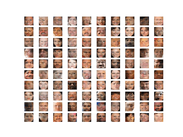
Example of Celebrity Faces Generated by a Generative Adversarial Network
How to Explore the Latent Space for Generated Faces
In this section, we will use our trained GAN model as the basis for exploring the latent space.
How to Load Model and Generate Faces
The first step is to load the saved model and confirm that it can generate plausible faces.
The model can be loaded using the load_model() function in the Keras API. We can then generate a number of random points in the latent space and use them as input to the loaded model to generate new faces. The faces can then be plotted.
The complete example is listed below.
# example of loading the generator model and generating images
from numpy import asarray
from numpy.random import randn
from numpy.random import randint
from keras.models import load_model
from matplotlib import pyplot

# generate points in latent space as input for the generator
def generate_latent_points(latent_dim, n_samples, n_classes=10):
	# generate points in the latent space
	x_input = randn(latent_dim * n_samples)
	# reshape into a batch of inputs for the network
	z_input = x_input.reshape(n_samples, latent_dim)
	return z_input

# create a plot of generated images
def plot_generated(examples, n):
	# plot images
	for i in range(n * n):
		# define subplot
		pyplot.subplot(n, n, 1 + i)
		# turn off axis
		pyplot.axis('off')
		# plot raw pixel data
		pyplot.imshow(examples[i, :, :])
	pyplot.show()

# load model
model = load_model('generator_model_030.h5')
# generate images
latent_points = generate_latent_points(100, 25)
# generate images
X  = model.predict(latent_points)
# scale from [-1,1] to [0,1]
X = (X + 1) / 2.0
# plot the result
plot_generated(X, 5)
Running the example first loads the saved model.
Then, 25 random points in the 100-dimensional latent space are created, provided to the generator model to create 25 images of faces, which are then plotted in a 5×5 grid.
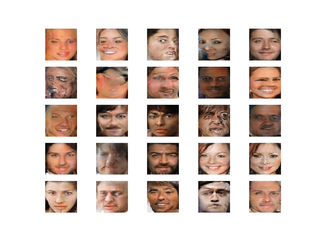
Plot of Randomly Generated Faces Using the Loaded GAN Model
How to Interpolate Between Generated Faces
Next, we can create an interpolation path between two points in the latent space and generate faces along this path.
The simplest interpolation we can use is a linear or uniform interpolation between two points in the latent space. We can achieve this using the linspace() NumPy function to calculate ratios of the contribution from two points, then enumerate these ratios and construct a vector for each ratio.
The interpolate_points() function below implements this and returns a series of linearly interpolated vectors between two points in latent space, including the first and last point.
# uniform interpolation between two points in latent space
def interpolate_points(p1, p2, n_steps=10):
	# interpolate ratios between the points
	ratios = linspace(0, 1, num=n_steps)
	# linear interpolate vectors
	vectors = list()
	for ratio in ratios:
		v = (1.0 - ratio) * p1 + ratio * p2
		vectors.append(v)
	return asarray(vectors)
We can then generate two points in the latent space, perform the interpolation, then generate an image for each interpolated vector.
The result will be a series of images that transition between the two original images. The example below demonstrates this for two faces.
# example of interpolating between generated faces
from numpy import asarray
from numpy.random import randn
from numpy.random import randint
from numpy import linspace
from keras.models import load_model
from matplotlib import pyplot

# generate points in latent space as input for the generator
def generate_latent_points(latent_dim, n_samples, n_classes=10):
	# generate points in the latent space
	x_input = randn(latent_dim * n_samples)
	# reshape into a batch of inputs for the network
	z_input = x_input.reshape(n_samples, latent_dim)
	return z_input

# uniform interpolation between two points in latent space
def interpolate_points(p1, p2, n_steps=10):
	# interpolate ratios between the points
	ratios = linspace(0, 1, num=n_steps)
	# linear interpolate vectors
	vectors = list()
	for ratio in ratios:
		v = (1.0 - ratio) * p1 + ratio * p2
		vectors.append(v)
	return asarray(vectors)

# create a plot of generated images
def plot_generated(examples, n):
	# plot images
	for i in range(n):
		# define subplot
		pyplot.subplot(1, n, 1 + i)
		# turn off axis
		pyplot.axis('off')
		# plot raw pixel data
		pyplot.imshow(examples[i, :, :])
	pyplot.show()

# load model
model = load_model('generator_model_030.h5')
# generate points in latent space
pts = generate_latent_points(100, 2)
# interpolate points in latent space
interpolated = interpolate_points(pts[0], pts[1])
# generate images
X = model.predict(interpolated)
# scale from [-1,1] to [0,1]
X = (X + 1) / 2.0
# plot the result
plot_generated(X, len(interpolated))
Running the example calculates the interpolation path between the two points in latent space, generates images for each, and plots the result.
You can see the clear linear progression in ten steps from the first face on the left to the final face on the right.
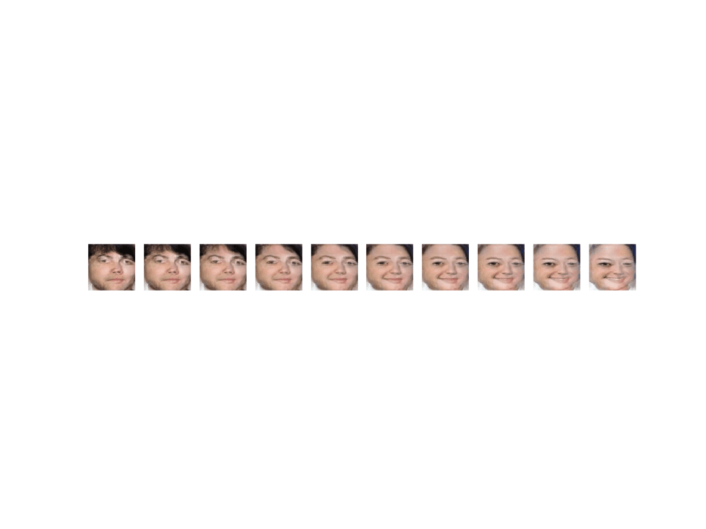
Plot Showing the Linear Interpolation Between Two GAN Generated Faces
We can update the example to repeat this process multiple times so we can see the transition between multiple generated faces on a single plot.
The complete example is listed below.
# example of interpolating between generated faces
from numpy import asarray
from numpy import vstack
from numpy.random import randn
from numpy.random import randint
from numpy import linspace
from keras.models import load_model
from matplotlib import pyplot

# generate points in latent space as input for the generator
def generate_latent_points(latent_dim, n_samples, n_classes=10):
	# generate points in the latent space
	x_input = randn(latent_dim * n_samples)
	# reshape into a batch of inputs for the network
	z_input = x_input.reshape(n_samples, latent_dim)
	return z_input

# uniform interpolation between two points in latent space
def interpolate_points(p1, p2, n_steps=10):
	# interpolate ratios between the points
	ratios = linspace(0, 1, num=n_steps)
	# linear interpolate vectors
	vectors = list()
	for ratio in ratios:
		v = (1.0 - ratio) * p1 + ratio * p2
		vectors.append(v)
	return asarray(vectors)

# create a plot of generated images
def plot_generated(examples, n):
	# plot images
	for i in range(n * n):
		# define subplot
		pyplot.subplot(n, n, 1 + i)
		# turn off axis
		pyplot.axis('off')
		# plot raw pixel data
		pyplot.imshow(examples[i, :, :])
	pyplot.show()

# load model
model = load_model('generator_model_030.h5')
# generate points in latent space
n = 20
pts = generate_latent_points(100, n)
# interpolate pairs
results = None
for i in range(0, n, 2):
	# interpolate points in latent space
	interpolated = interpolate_points(pts[i], pts[i+1])
	# generate images
	X = model.predict(interpolated)
	# scale from [-1,1] to [0,1]
	X = (X + 1) / 2.0
	if results is None:
		results = X
	else:
		results = vstack((results, X))
# plot the result
plot_generated(results, 10)
Running the example creates 10 different face starting points and 10 matching face endpoints, and the linear interpolation between each.
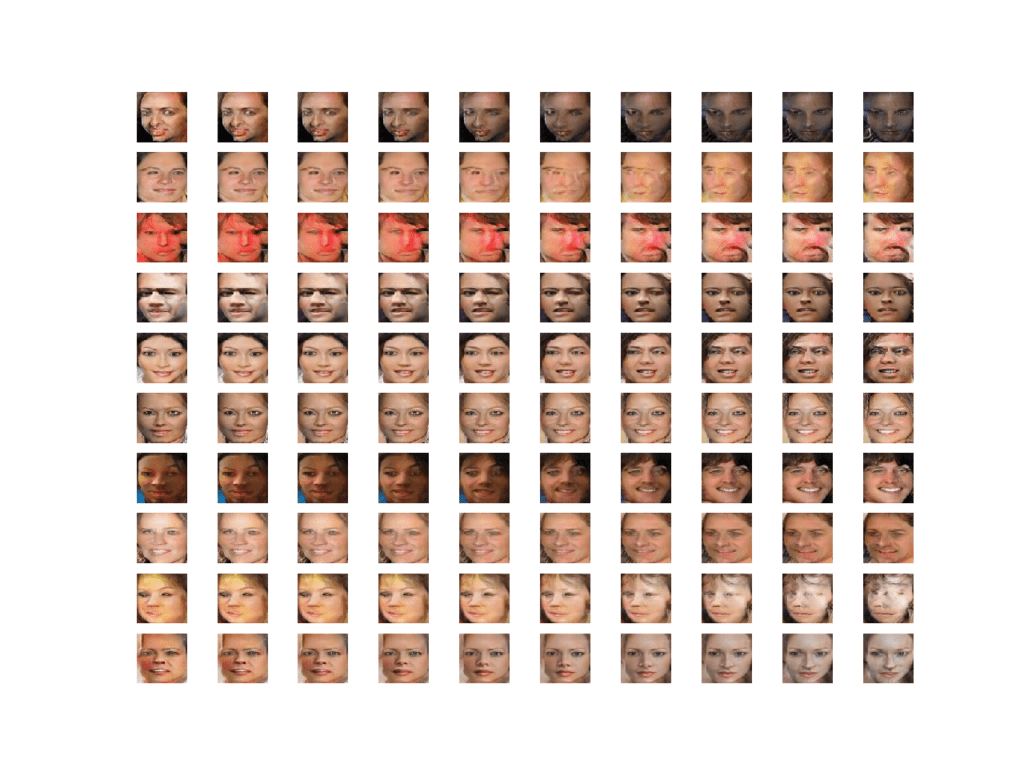
Plot Showing Multiple Linear Interpolations Between Two GAN Generated Faces
In these cases, we have performed a linear interpolation which assumes that the latent space is uniformly distributed hypercube. Technically, our chosen latent space is a 100-dimension hypersphere or multimodal Gaussian distribution.
There is a mathematical function called the spherical linear interpolation function, or ‘Slerp,’ that should be used when interpolating this space to ensure the curving of the space is taken into account. For more details, I recommend reading the Issue on Linear Interpolation in Soumith Chintala’s dcgan.torch project. In that project, an implementation of the Slerp function for Python is provided that we can use as the basis for our own Slerp function, provided below:
# spherical linear interpolation (slerp)
def slerp(val, low, high):
	omega = arccos(clip(dot(low/norm(low), high/norm(high)), -1, 1))
	so = sin(omega)
	if so == 0:
		# L'Hopital's rule/LERP
		return (1.0-val) * low + val * high
	return sin((1.0-val)*omega) / so * low + sin(val*omega) / so * high
This function can be called from our interpolate_points() function instead of performing the manual linear interpolation.
The complete example with this change is listed below.
# example of interpolating between generated faces
from numpy import asarray
from numpy import vstack
from numpy.random import randn
from numpy.random import randint
from numpy import arccos
from numpy import clip
from numpy import dot
from numpy import sin
from numpy import linspace
from numpy.linalg import norm
from keras.models import load_model
from matplotlib import pyplot

# generate points in latent space as input for the generator
def generate_latent_points(latent_dim, n_samples, n_classes=10):
	# generate points in the latent space
	x_input = randn(latent_dim * n_samples)
	# reshape into a batch of inputs for the network
	z_input = x_input.reshape(n_samples, latent_dim)
	return z_input

# spherical linear interpolation (slerp)
def slerp(val, low, high):
	omega = arccos(clip(dot(low/norm(low), high/norm(high)), -1, 1))
	so = sin(omega)
	if so == 0:
		# L'Hopital's rule/LERP
		return (1.0-val) * low + val * high
	return sin((1.0-val)*omega) / so * low + sin(val*omega) / so * high

# uniform interpolation between two points in latent space
def interpolate_points(p1, p2, n_steps=10):
	# interpolate ratios between the points
	ratios = linspace(0, 1, num=n_steps)
	# linear interpolate vectors
	vectors = list()
	for ratio in ratios:
		v = slerp(ratio, p1, p2)
		vectors.append(v)
	return asarray(vectors)

# create a plot of generated images
def plot_generated(examples, n):
	# plot images
	for i in range(n * n):
		# define subplot
		pyplot.subplot(n, n, 1 + i)
		# turn off axis
		pyplot.axis('off')
		# plot raw pixel data
		pyplot.imshow(examples[i, :, :])
	pyplot.show()

# load model
model = load_model('generator_model_030.h5')
# generate points in latent space
n = 20
pts = generate_latent_points(100, n)
# interpolate pairs
results = None
for i in range(0, n, 2):
	# interpolate points in latent space
	interpolated = interpolate_points(pts[i], pts[i+1])
	# generate images
	X = model.predict(interpolated)
	# scale from [-1,1] to [0,1]
	X = (X + 1) / 2.0
	if results is None:
		results = X
	else:
		results = vstack((results, X))
# plot the result
plot_generated(results, 10)
The result is 10 more transitions between generated faces, this time using the correct Slerp interpolation method.
The difference is subtle but somehow visually more correct.
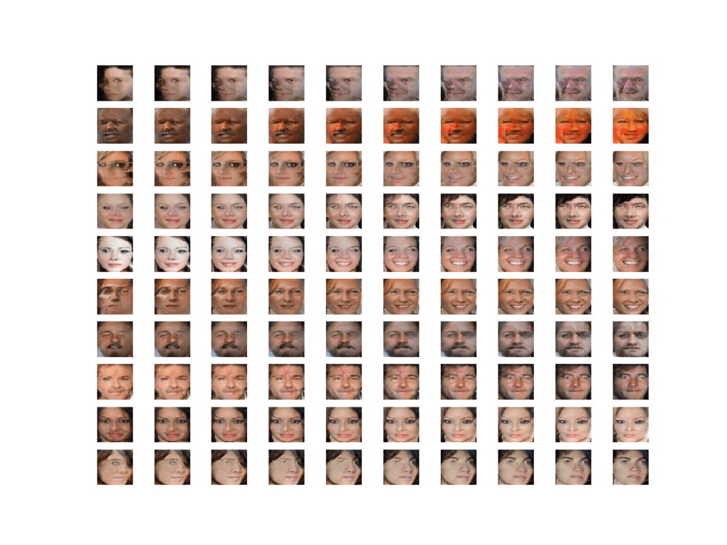
Plot Showing Multiple Seraphically Linear Interpolation Between Two GAN Generated Faces
How to Perform Vector Arithmetic With Faces
Finally, we can explore the latent space by performing vector arithmetic with the generated faces
First, we must generate a large number of faces and save both the faces and their corresponding latent vectors. We can then review the plot of generated faces and select faces with features we’re interested in, note their index (number), and retrieve their latent space vectors for manipulation.
The example below will load the GAN model and use it to generate 100 random faces.
# example of loading the generator model and generating images
from numpy import asarray
from numpy.random import randn
from numpy.random import randint
from keras.models import load_model
from matplotlib import pyplot
from numpy import savez_compressed

# generate points in latent space as input for the generator
def generate_latent_points(latent_dim, n_samples, n_classes=10):
	# generate points in the latent space
	x_input = randn(latent_dim * n_samples)
	# reshape into a batch of inputs for the network
	z_input = x_input.reshape(n_samples, latent_dim)
	return z_input

# create a plot of generated images
def plot_generated(examples, n):
	# plot images
	for i in range(n * n):
		# define subplot
		pyplot.subplot(n, n, 1 + i)
		# turn off axis
		pyplot.axis('off')
		# plot raw pixel data
		pyplot.imshow(examples[i, :, :])
	pyplot.savefig('generated_faces.png')
	pyplot.close()

# load model
model = load_model('generator_model_030.h5')
# generate points in latent space
latent_points = generate_latent_points(100, 100)
# save points
savez_compressed('latent_points.npz', latent_points)
# generate images
X  = model.predict(latent_points)
# scale from [-1,1] to [0,1]
X = (X + 1) / 2.0
# save plot
plot_generated(X, 10)
Running the example loads the model, generates faces, and saves the latent vectors and generated faces.
The latent vectors are saved to a compressed NumPy array with the filename ‘latent_points.npz‘. The 100 generated faces are plotted in a 10×10 grid and saved in a file named ‘generated_faces.png‘.
In this case, we have a good collection of faces to work with. Each face has an index that we can use to retrieve the latent vector. For example, the first face is 1, which corresponds to the first vector in the saved array (index 0).
We will perform the operation:
smiling woman - neutral woman + neutral man = smiling man
Therefore, we need three faces for each of smiling woman, neutral woman, and neutral man.
In this case, we will use the following indexes in the image:
- Smiling Woman: 92, 98, 99
- Neutral Woman: 9, 21, 79
- Neutral Man: 10, 30, 45
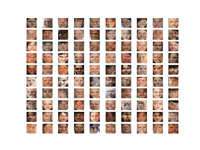
Plot of 100 Generated Faces Used as the Basis for Vector Arithmetic with Faces
Now that we have latent vectors to work with and a target arithmetic, we can get started.
First, we can specify our preferred images and load the saved NumPy array of latent points.
# retrieve specific points
smiling_woman_ix = [92, 98, 99]
neutral_woman_ix = [9, 21, 79]
neutral_man_ix = [10, 30, 45]
# load the saved latent points
data = load('latent_points.npz')
points = data['arr_0']
Next, we can retrieve each vector and calculate the average for each vector type (e.g. smiling woman). We could perform vector arithmetic with single images directly, but we will get a more robust result if we work with an average of a few faces with the desired property.
The average_points() function below takes the loaded array of latent space points, retrieves each, calculates the average, and returns all of the vectors.
# average list of latent space vectors
def average_points(points, ix):
	# convert to zero offset points
	zero_ix = [i-1 for i in ix]
	# retrieve required points
	vectors = points[zero_ix]
	# average the vectors
	avg_vector = mean(vectors, axis=0)
	# combine original and avg vectors
	all_vectors = vstack((vectors, avg_vector))
	return all_vectors
We can now use this function to retrieve all of the required points in latent space and generate images.
# average vectors
smiling_woman = average_points(points, smiling_woman_ix)
neutral_woman = average_points(points, neutral_woman_ix)
neutral_man = average_points(points, neutral_man_ix)
# combine all vectors
all_vectors = vstack((smiling_woman, neutral_woman, neutral_man))
# generate images
images = model.predict(all_vectors)
# scale pixel values
images = (images + 1) / 2.0
plot_generated(images, 3, 4)
Finally, we can use the average vectors to perform vector arithmetic in latent space and plot the result.
# smiling woman - neutral woman + neutral man = smiling man
result_vector = smiling_woman[-1] - neutral_woman[-1] + neutral_man[-1]
# generate image
result_vector = expand_dims(result_vector, 0)
result_image = model.predict(result_vector)
# scale pixel values
result_image = (result_image + 1) / 2.0
pyplot.imshow(result_image[0])
pyplot.show()
Tying this together, the complete example is listed below.
# example of loading the generator model and generating images
from numpy import asarray
from numpy.random import randn
from numpy.random import randint
from keras.models import load_model
from matplotlib import pyplot
from numpy import load
from numpy import mean
from numpy import vstack
from numpy import expand_dims

# average list of latent space vectors
def average_points(points, ix):
	# convert to zero offset points
	zero_ix = [i-1 for i in ix]
	# retrieve required points
	vectors = points[zero_ix]
	# average the vectors
	avg_vector = mean(vectors, axis=0)
	# combine original and avg vectors
	all_vectors = vstack((vectors, avg_vector))
	return all_vectors

# create a plot of generated images
def plot_generated(examples, rows, cols):
	# plot images
	for i in range(rows * cols):
		# define subplot
		pyplot.subplot(rows, cols, 1 + i)
		# turn off axis
		pyplot.axis('off')
		# plot raw pixel data
		pyplot.imshow(examples[i, :, :])
	pyplot.show()

# load model
model = load_model('generator_model_030.h5')
# retrieve specific points
smiling_woman_ix = [92, 98, 99]
neutral_woman_ix = [9, 21, 79]
neutral_man_ix = [10, 30, 45]
# load the saved latent points
data = load('latent_points.npz')
points = data['arr_0']
# average vectors
smiling_woman = average_points(points, smiling_woman_ix)
neutral_woman = average_points(points, neutral_woman_ix)
neutral_man = average_points(points, neutral_man_ix)
# combine all vectors
all_vectors = vstack((smiling_woman, neutral_woman, neutral_man))
# generate images
images = model.predict(all_vectors)
# scale pixel values
images = (images + 1) / 2.0
plot_generated(images, 3, 4)
# smiling woman - neutral woman + neutral man = smiling man
result_vector = smiling_woman[-1] - neutral_woman[-1] + neutral_man[-1]
# generate image
result_vector = expand_dims(result_vector, 0)
result_image = model.predict(result_vector)
# scale pixel values
result_image = (result_image + 1) / 2.0
pyplot.imshow(result_image[0])
pyplot.show()
Running the example first loads the points in latent space for our specific images, calculates the average of the points, and generates the faces for the points.
We can see that, indeed, our selected faces were retrieved correctly and that the average of the points in the vector space captures the salient feature we are going for on each line (e.g. smiling woman, neutral woman, etc.).
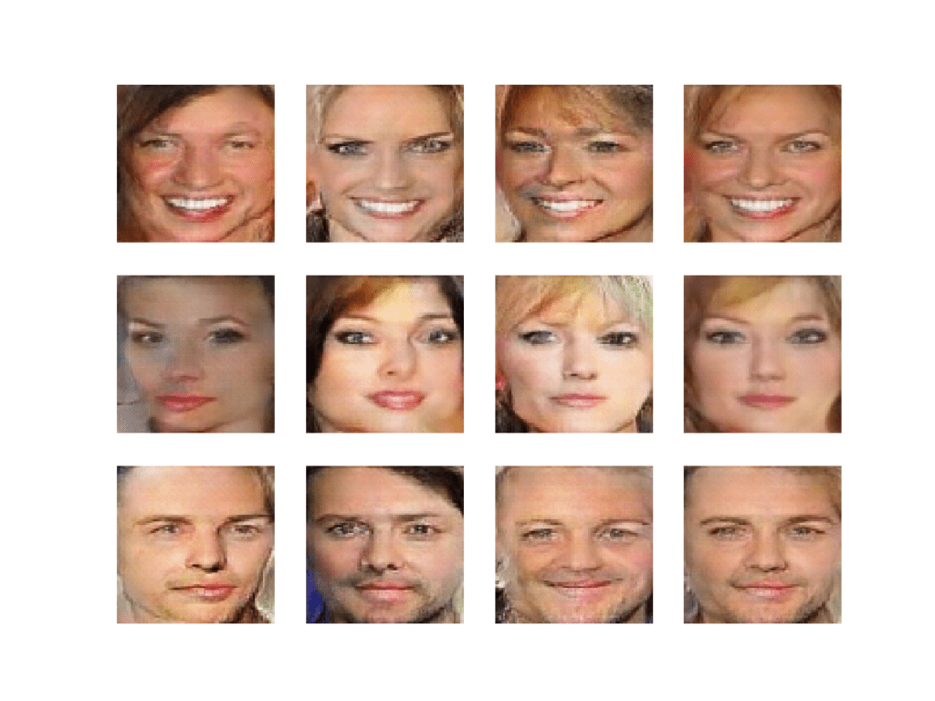
Plot of Selected Generated Faces and the Average Generated Face for Each Row
Next, vector arithmetic is performed and the result is a smiling man, as we would expect.
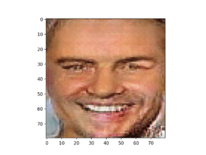
Plot of the Resulting Generated Face Based on Vector Arithmetic in Latent Space
Extensions
This section lists some ideas for extending the tutorial that you may wish to explore.
- Additional Arithmetic. Try arithmetic with different image features or different arithmetic and review the results of the generated faces.
- Additional Interpolation. Try interpolating between three or more points in latent space and review the results of the generated faces.
- Tune Model. Update the GAN model configuration so that training is more stable and better quality faces can be generated.
If you explore any of these extensions, I’d love to know.
Post your findings in the comments below.
Further Reading
This section provides more resources on the topic if you are looking to go deeper.
Books
- Chapter 20. Deep Generative Models, Deep Learning, 2016.
- Chapter 8. Generative Deep Learning, Deep Learning with Python, 2017.
Papers
- Generative Adversarial Networks, 2014.
- Unsupervised Representation Learning with Deep Convolutional Generative Adversarial Networks, 2015
- Tutorial: Generative Adversarial Networks, NIPS, 2016.
- Joint Face Detection and Alignment Using Multitask Cascaded Convolutional Networks, 2016.
API
- Keras Datasets API.
- Keras Sequential Model API
- Keras Convolutional Layers API
- How can I “freeze” Keras layers?
- MatplotLib API
- NumPy Random sampling (numpy.random) API
- NumPy Array manipulation routines
Articles
- Large-scale CelebFaces Attributes (CelebA) Dataset.
- CelebFaces Attributes (CelebA) Dataset, Kaggle.
- Celebrity Face Generation using GANs (Tensorflow Implementation), 2018.
- MTCNN Face Detection Project, GitHub.
- linear interpolation?, dcgan.torch Project, GitHub.
Summary
In this tutorial, you discovered how to develop a generative adversarial network for face generation and explore the structure of latent space and the effect on generated faces.
Specifically, you learned:
- How to develop a generative adversarial network for generating faces.
- How to interpolate between points in latent space and generate images that morph from one face to another.
- How to perform vector arithmetic in latent space and achieve targeted results in the resulting generated faces.
Do you have any questions?
Ask your questions in the comments below and I will do my best to answer.
The post How to Explore the GAN Latent Space When Generating Faces appeared first on Machine Learning Mastery.
