Author: Marco Tavora
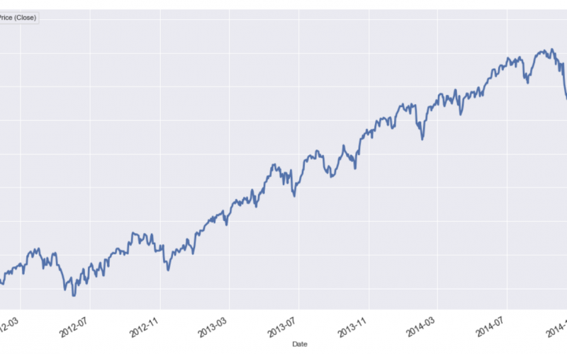
In financial markets, two of the most common trading strategies used by investors are the momentum and mean reversion strategies. If a stock exhibits momentum (or trending behavior as shown in the figure below), its price on the current period is more likely to increase (decrease) if it has already increased (decreased) on the previous period.
Below, a section of the time series of the S&P 500 Index or SPY is shown. This is an example of trending behavior.
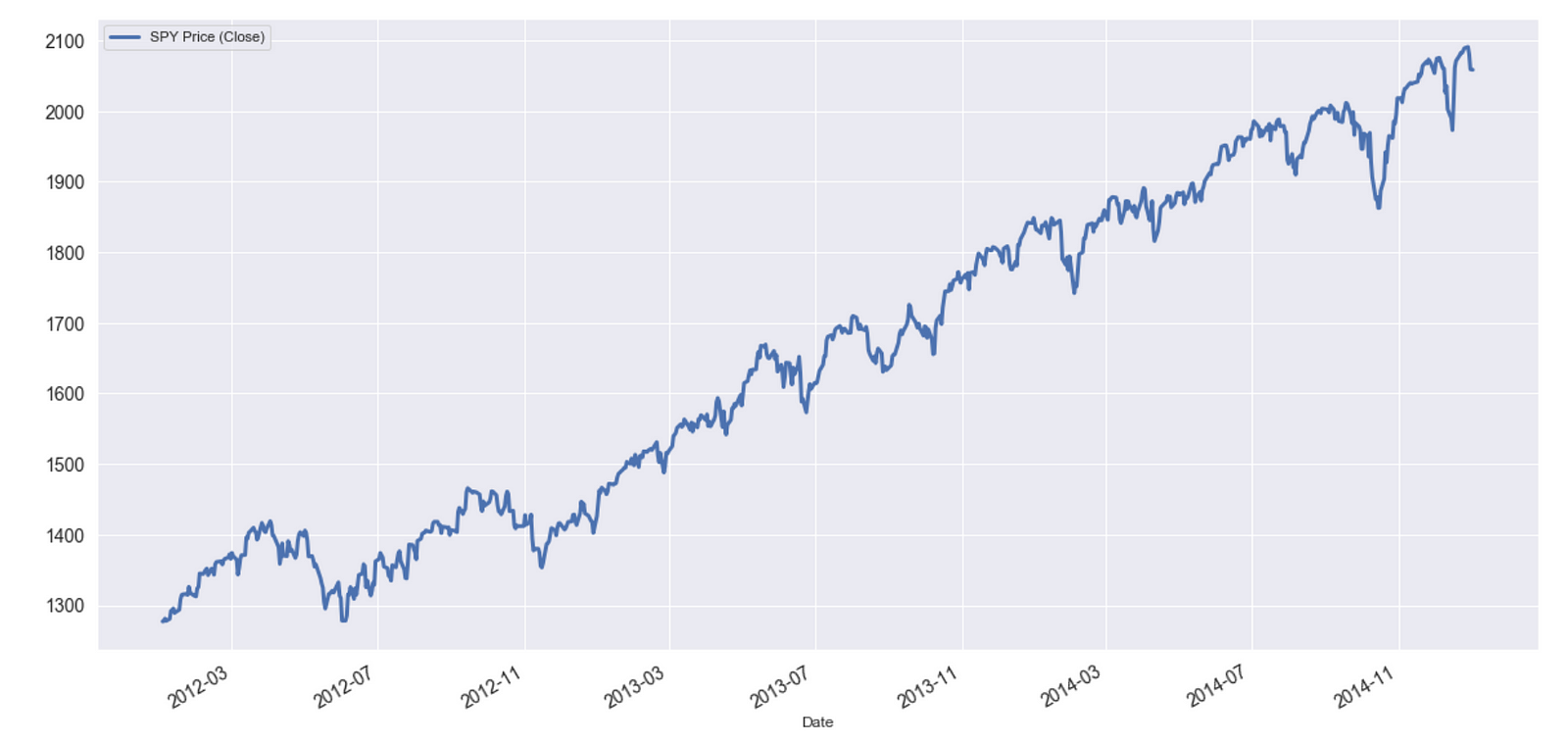
When the return of a stock at time t depends in some way on the return at the previous time t–1, the returns are said to be autocorrelated. In the momentum regime, returns are positively correlated.
In contrast, the price of a mean-reverting stock fluctuates randomly around its historical mean and displays a tendency to revert to it. When there is mean reversion, if the price increased (decreased) in the current period, it is more likely to decrease (increase) in the next one.
A section of the time series of log returns of the Apple stock (adjusted closing price), shown below, is an example of mean-reverting behavior.
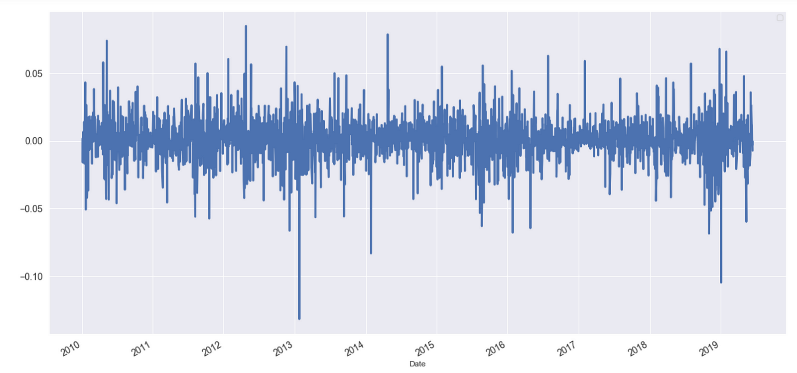
Note that, since the two regimes occur in different time frames (trending behavior usually occurs in larger timescales), they can, and often do, coexist.
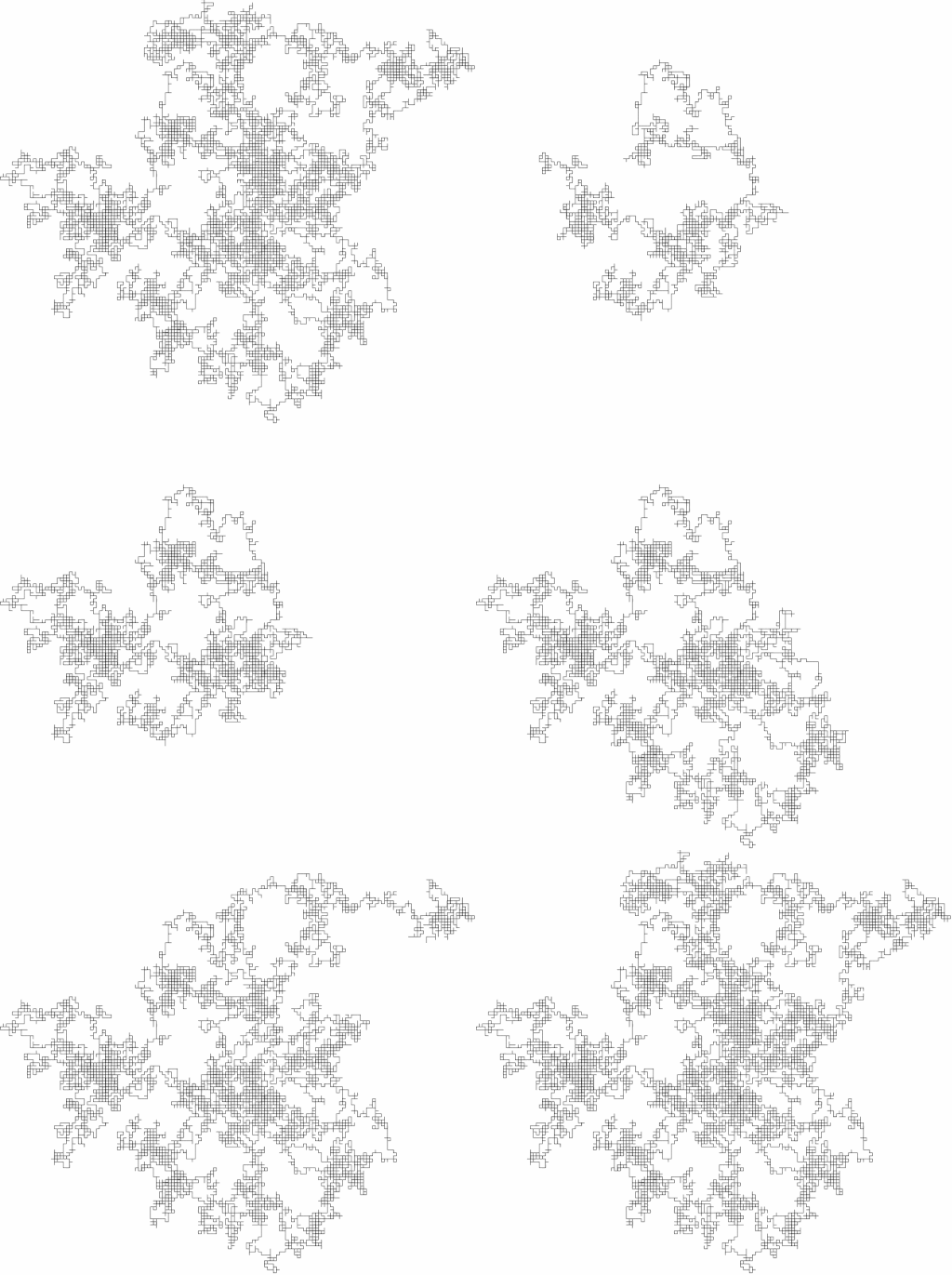
In both regimes, the current price contains useful information about the future price. In fact, trading strategies can only generate profit if asset prices are either trending or mean-reverting since, otherwise, prices are following what is known as a random walk (see the animation below).
Mean-Reverting Time Series
Stock prices rarely display mean-reverting behavior. In the vast majority of cases, they follow random walks (their corresponding returns, however, are mean-reverting and fluctuate randomly around zero). Mean-reverting price series can, however, be synthesized by combining different stocks to build a cointegrated portfolio (see this reference for more details) which displays the property of stationarity (a lot more about this below). Though stationarity can be identified using a variety of well-known standard statistical tests, in this article, I will focus on one powerful type of analysis based on the so-called Hurst exponent, which is related to the fractal exponent of the price time series. The Hurst exponent provides a way to measure the amount by which a financial time series deviates from a random walk. It is a surprisingly simple tool that can help investors determine which strategy to apply.
Stationarity
In this article, for practical purposes, I will informally use the terms mean-reverting and stationary interchangeably. Now, suppose the price of a given stock, which I will represent by S(t), exhibits mean-reverting behavior. This behavior can be more formally described the following stochastic differential equation (SDE)

SDE describing a mean-reverting process.
Here, the symbols

are, respectively, the stock price at time t, a Wiener process (or Brownian motion) at time t, the rate of reversion θ to the mean, the equilibrium or mean value of the process μ and its volatility σ. According to this SDE, the variation of the price at t+1 is proportional to the difference between the price at time t and the mean. As we can see, the price variation is more likely to be positive (negative) if the price is smaller (greater) than the mean. A well-known special case of this SDE is the so-called Ornstein-Uhlenbeck process. The Ornstein-Uhlenbeck process was named after the Dutch physicist Leonard Ornstein and the Dutch-American physicist George Eugene Uhlenbeck (see figure below).

Two of the best-known tests for (non-)stationarity are the Dickey-Fuller test (DF) and the Augmented Dickey-Fuller (ADF) tests.
Dickey-Fuller and Augmented Dickey-Fuller Tests: A Bird’s-Eye View
The ADF test is an extension of the DF test, so let us first understand the latter. It can be illustrated as follows. Consider the simple model given by:

where S(t) are stock prices varying in time, ρ is a coefficient and the last term is an error term. The null hypothesis here is that ρ=1. Since under the null hypothesis both S(t) and S(t-1) are non-stationary, the central limit theorem is violated and one has to resort to the following trick.
The Dickey-Fuller test is named for the statisticians Wayne Fuller and David Dickey (picture below). The ADF is an extension of this test for more complex time series models.

Defining the first difference and the parameter δ as follows

the regression model can be conveniently rewritten as:

The Dickey-Fuller then tests the hypothesis (technically the null hypothesis) that

where the distribution of δ was tabulated by Wayne Fuller and David Dickey.
The logic behind the DF test can be heuristically understood as follows. If S(t) is stationary it tends to return to some constant mean (or possibly a trend that evolves deterministically) which means that larger values are likely to follow smaller ones and vice-versa. That makes the current value of the series a strong predictor of the following value and we would have δ < 0. If S(t) is non-stationary future changes do not depend on the current values (for example, if the process is a random walk, the current value does not affect the next).
The ADF test follows a similar procedure but it is applied to a more complex hence more complete model given by:

Here, α is a real constant, β is the coefficient of the trend in time (a drift term), the δs are the coefficients of the differences

where p is the lag order of the process and the last term is the error. The test statistic here is

where the denominator is the standard error of the regression fit. The distribution of this test statistic was also tabulated by Dickey and Fuller. As in the case of the DF test, we expect γ<0. Details on how to carry on the test can be found in any time series book.
Python Code
The following Python snippet illustrates the application of the ADF test to Apple stocks prices. Though stock prices are rarely mean reverting, stock log returns usually are. This Python code obtains log differences, plots the result and applies the ADF test.
The plot is the following:
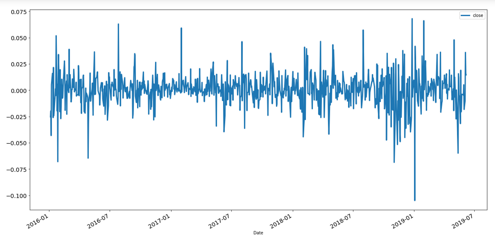
Log returns for Apple stocks.
The output from the ADF test is:
Augmented Dickey-Fuller test statistic: -28.653611206757994
p-value: 0.0
Critical Values:

        1%: -3.4379766581448803

        5%: -2.8649066016199836

        10%: -2.5685626352082207
In general, we are more likely to reject the null hypothesis, according to which the series is non-stationary (it has a unit root), the “more negative” the ADF test statistic is. The above test corroborates the hypothesis that the log return series is indeed stationary. The result shows that the statistic value of around -28.65 is less than -3.438 at 1%, the significance level with which we can reject the null hypothesis (see this link for more details).
The Hurst Exponent
There is an alternative way to investigate the presence of mean reversion or trending behavior in a process. As will be explained in detail shortly, this can be done by analyzing the diffusion speed of the series and comparing it with the diffusion rate of a random walk. This procedure will lead us to the concept of the Hurst exponent which, as we shall see, is closely connected to fractal exponents.
Though applications of the Hurst exponent can be found in multiple areas of mathematics, our focus here will be in two of them only, namely fractals and long memory processes.
Fractals
A fractal can be defined as follows:
“A curve or geometric figure, each part of which has the same statistical character as the whole. Fractals are useful in modeling structures (such as eroded coastlines or snowflakes) in which similar patterns recur at progressively smaller scales, and in describing partly random or chaotic phenomena such as crystal growth, fluid turbulence, and galaxy formation.”
An example of a fractal is the Sierpinski triangle shown in the figure below.

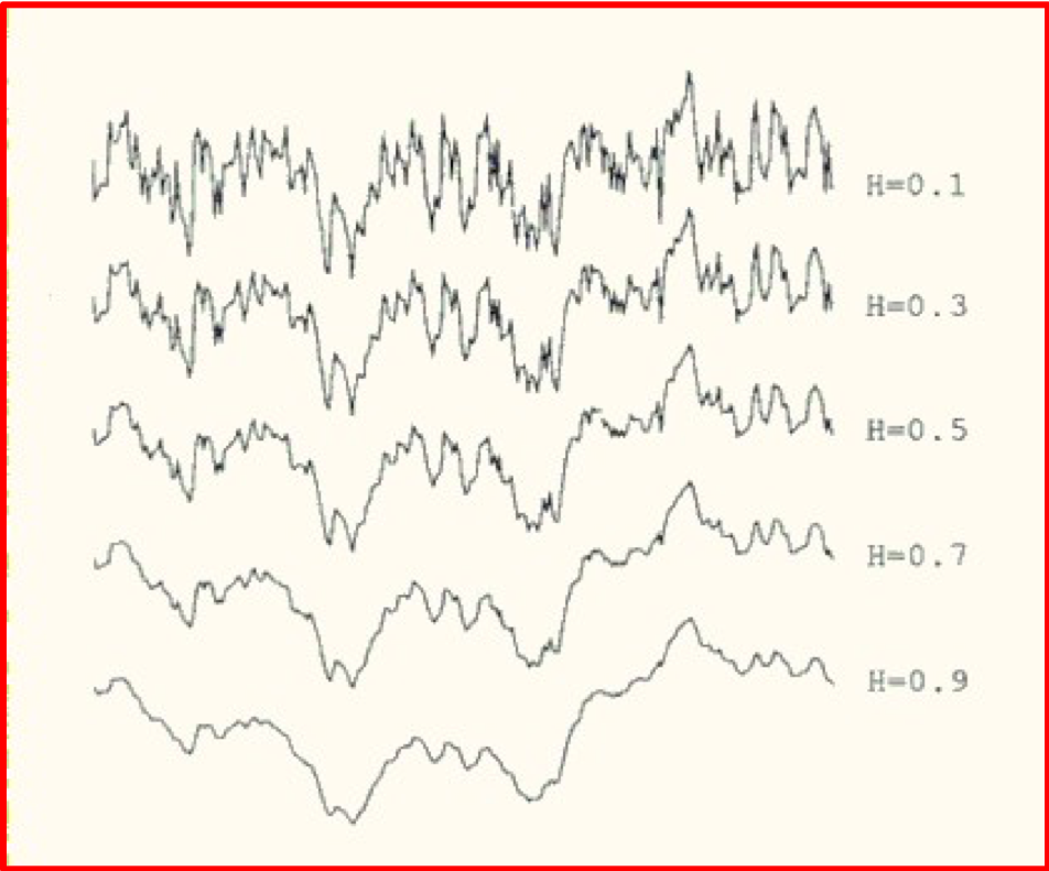
The “fractal dimension” which measures the roughness of a surface, has the following simple relation with H,

We see that large Hurst exponents are associated with small fractal dimensions i.e. with smoother curves or surfaces. An example is shown below. This illustration, taken from this article, clearly shows that as H increases, the curve indeed gets smoother.
Fractals have a property called self-similarity. One type of self-similarity which occurs in several branches of engineering and applied mathematics is called statistical self-similarity. In data sets displaying this kind of self-similarity, any subsection is statistically similar to the full set. Probably the most famous example of statistical self-similarity is found in coastlines.
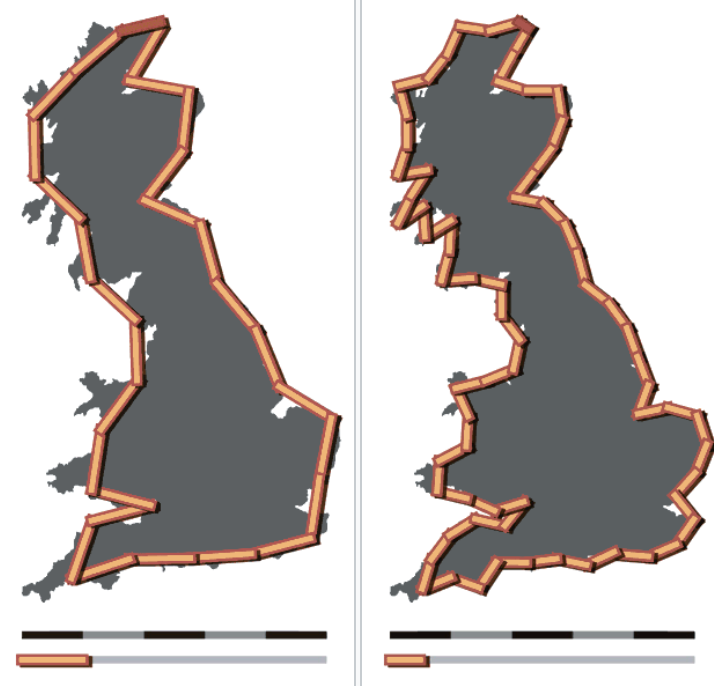
In 1967, Benoit Mandelbrot, one of the fathers of the field of fractal geometry, published on Science Magazine a seminal paper entitled “How Long Is the Coast of Britain? Statistical Self-Similarity and Fractional Dimension” where he discussed the properties of fractals such as self-similarity and fractional (Hausdorff) dimensions. The picture above shows an example of the coastline paradox. According to it, if one measures coastlines using different units one obtains different results.
Long Range Dependence
One important kind of departure from random walks occurs when processes have long-range dependence. These processes display a high persistence degree: past events are nontrivially correlated with future events even if they are very far apart. One example, conceived by Granger, Joyeux, and Hosking, is given by the following fractionally differenced time series:

where L is the usual lag operator, the exponent d is noninteger and ϵ is an error term. Using a simple binomial expansion this equation can be expressed in terms of Gamma functions

Comparing the autocorrelation function of a simple AR(1) process we find that the autocorrelation function of the latter has a much slower decay rate than the one from the former. For example, for a lag of τ~25,

whereas the corresponding value of the autocorrelation function of the fractionally differenced process is ~-0.17.
Origins of the Hurst Exponent
Though most recent developments regarding methods of estimation of the Hurst exponent are coming from the mathematics of fractals and chaos theory, the Hurst exponent was curiously first used in the field of hydrology, which is mainly concerned with water distribution, quality, and its movement in relation to land. Furthermore, recent tests for long term dependence in financial time series are based on a statistic called Rescaled Range (see below), originally developed by the English hydrologist Harold Hurst. The front page of Hurst’s original paper is shown below.

Hurst Exponent and Anomalous Diffusion
One way to gain some understanding of the nature of a price series is to analyze its speed of diffusion. Diffusion is a widely used concept which describes the “spreading out” of some object (which could be an idea, the price of an asset, a disease, etc) from a location where its concentration is higher than in most other places.
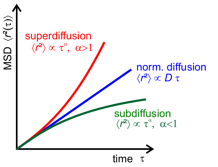
The plot shows how the mean squared displacement varies with the elapsed time τ for three types of diffusion (source).
Diffusion can be measured studying how the variance depends on the difference between subsequent measurements:

In this expression, τ is the time interval between two measurements and x is a generic function of the price S(t). This function is often chosen to be the log price:

It is a well-known fact that the variance of stock price returns depends strongly on the frequency one chooses to measure it. Measurements at high frequencies say, in 1-minute intervals, differ significantly from daily measurements.
If stock prices follow, which is not always the case (in particular for daily returns), a geometric random walk (or equivalently a geometric Brownian motion or GBM), the variance would vary linearly with the lag τ

and the returns would be normally distributed. However, when there are small deviations from a pure random walk, as it often occurs, the variance for a given lag τ is not proportional to the τ anymore but instead, it acquires an anomalous exponent

The anomalous exponent is proportional to the Hurst exponent (source).
The parameter H is the so-called Hurst exponent. Both mean-reverting and trending stocks are characterized by

Daily returns satisfying this equation do not have a normal distribution. Instead, the distribution has fatter tails and thinner and higher peaks around the mean.
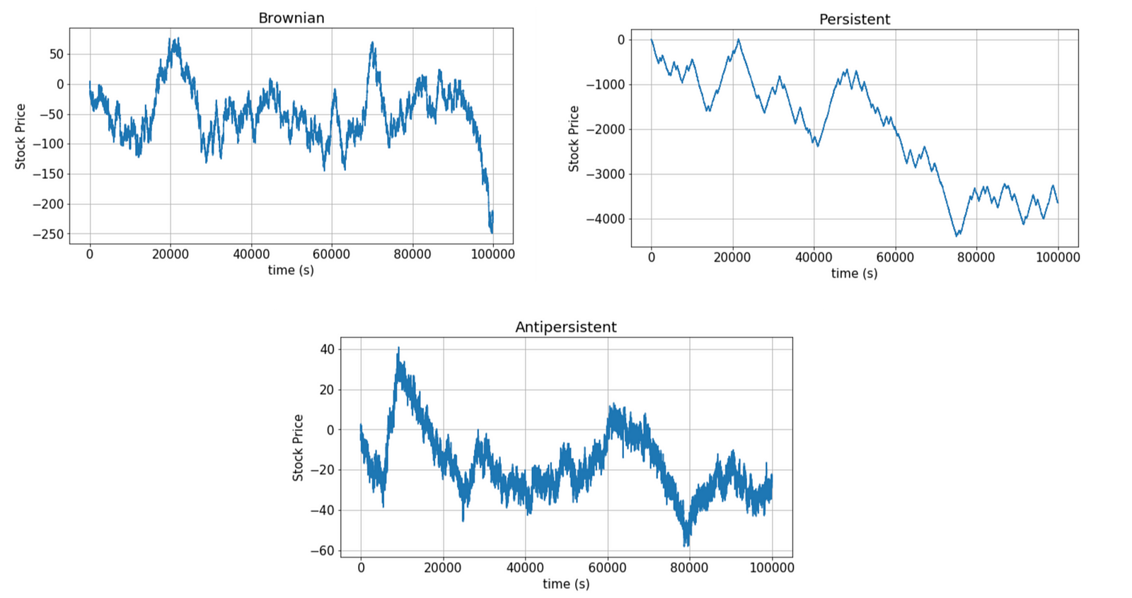
The Hurst exponent can be used to distinguish three possible market regimes:
- If H < 0.5, the time series is mean reverting or stationary. The log-price volatility increases at a slower rate compared to normal diffusion associated with geometric Brownian motion. In this case, the series displays what is known as antipersistence (long-term switching between high and low values in adjacent points)
- If H > 0.5, the series displays trending behavior and it is characterized by the presence of persistent behavior (long-term positive autocorrelation i.e. high values are likely to follow high values)
- The H = 0.5 case corresponds to a Geometric Brownian Motion
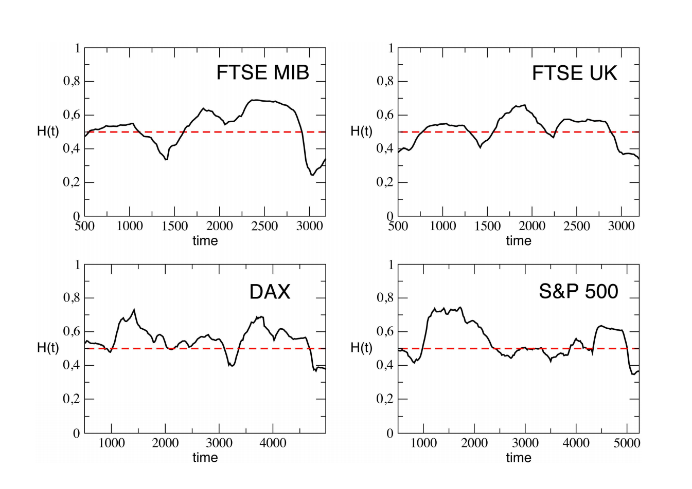
The Hurst exponent, therefore, measures the level of persistence of a time series and can be used to identify the market state: if at some time scale, the Hurst exponent changes, this may signal a shift from a mean reversion to a momentum regime or vice versa.

Relations between market regimes and the Hurst exponent.
The Hurst exponent, therefore, measures the level of persistence of a time series and can be used to identify the market state.
Examples of each case are plotted below:
In the next figure, we see how the Hurst exponent can vary with time indicating a change in regime.
Autocorrelation
The autocorrelation function for the stock price S(t) is defined as follows:

Processes with autocorrelations that decay very slowly are termed long memory processes. Such processes have some memory of past events (past events have a decaying influence on future events). Long memory processes are characterized by autocorrelation functions ρ(τ) with power-law decay

The relation between α and the Hurst exponent is

Note that as H approaches 1, the decay becomes slower and slower since the exponent α approaches zero, indicating “persistent behavior”. It often happens that processes that appear random at first, are actually long memory processes, having Hurst exponents within the open interval

Those processes are often referred to as fractional Brownian motion (fBm) or black noise, a generalization of Brownian motion.
Important Issues with Using the Variance to Estimate the Hurst
To obtain the variance dependence on τ, we must repeat the same calculation for many lags, and extract the slope of the logarithmic plot of the result. As we will see now, the value of H depends strongly on our choices of lags. This section is based on the analysis found in this blog post.
Let us consider the S&P 500 Index SPY and estimate the Hurst exponent for different lags. We first run this code, which takes the range of lags to be from 2 to 20.
We obtain the following value for H:
hurst = 0.43733191005891303
As previously explained, this value of H indicates a mean-reverting regime, albeit rather mild. The same code with lags 300–400, gives:
hurst = 0.6107941846903405
This value of H indicates the presence of a trending regime. We see, therefore, that the choice of lags strongly affects the value of the Hurst exponent. This means that this time series is neither purely mean-reverting nor trending, but changes behavior or shifts regimes depending on whether one measures it over short intervals or over the long term. Furthermore, as noted here, since these conclusions are far from obvious for the naked eye, we conclude that this analysis based on the Hurst exponent can give important insights.
Long-Range Dependence and the Rescaled Range
The presence of long term anomalous behavior of stock returns was noticed in 1971 by Mandelbrot (picture below).

To test for such long-range dependence, Mandelbrot used the Rescaled Range or R/S test statistic, briefly mentioned above. The R/S statistic is the range of partial sums of deviations of a series from its mean rescaled by the standard deviation (see this book for more details). Mandelbrot and others showed that using the R/S statistic leads to far superior results when compared with other methods such as the analysis of autocorrelations, variance ratios, and spectral decomposition, though it does have shortcomings, such as sensitivity to short-range dependence (for more details, see this article and this excellent blog post).
The R/S statistic can be obtained as follows. Consider for example the following time series of stock returns of length n

The partial sum of the first k deviations from the mean is given by:

The R/S statistic is proportional to the difference between the maximum and minimum of such sums where k ∈ [1,n]:

The denominator σ(n) is the maximum likelihood standard deviation estimator. The rescaled range and the number n of observations have the following relation

where H is the Hurst exponent. This scaling behavior was first used by Mandelbrot and Wallis to find the presence of long-range dependence. Since the relation between the rescaled range and the number of observations is polynomial, one can calculate the value of H with a simple log-log plot since

In the plot below, the Hurst exponent is estimated to be around 0.53 which approximately corresponds to a random walk. The corresponding code uses the hurst library (the link to the Github repo is here).
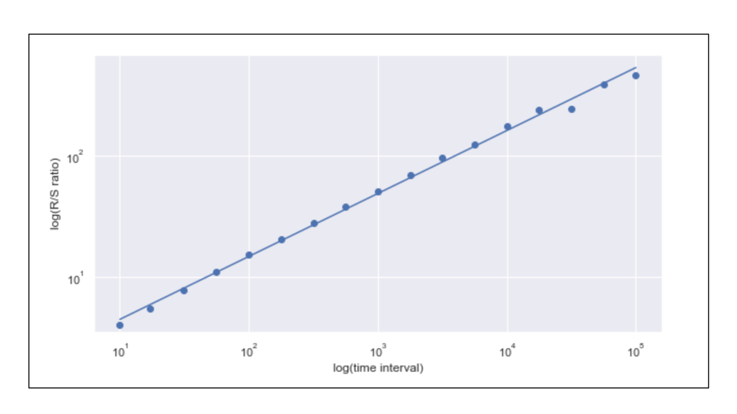
Estimation of the Hurst exponent gives H~0.5183. The code uses the Github repo found here. There are other methods to obtain the Hurst. You can check this article for more details on that.
Conclusions and Outlook
We saw that using the concept of the Hurst exponent can lead to very useful insights about the market regime. With that information in hand, one can decide which of the two strategies, mean reversion or momentum, is more appropriate to adopt.
In short, the value of the Hurst exponent identifies if the time series has some memory of past events. The fact that the value of the Hurst is not always equal to 1/2 shows that the efficient market hypothesis, according to which markets are completely unpredictable is often violated. Properly identifying such anomalies can in principle be extremely useful for building efficient trading strategies.
My Github and personal website www.marcotavora.me have (hopefully) some other interesting stuff about data science and quantitative finance.
This article was originally published on Towards Data Science.
