Author: Jason Brownlee
Generative Adversarial Networks, or GANs, are an architecture for training generative models, such as deep convolutional neural networks for generating images.
The conditional generative adversarial network, or cGAN for short, is a type of GAN that involves the conditional generation of images by a generator model. Image generation can be conditional on a class label, if available, allowing the targeted generated of images of a given type.
The Auxiliary Classifier GAN, or AC-GAN for short, is an extension of the conditional GAN that changes the discriminator to predict the class label of a given image rather than receive it as input. It has the effect of stabilizing the training process and allowing the generation of large high-quality images whilst learning a representation in the latent space that is independent of the class label.
In this tutorial, you will discover how to develop an auxiliary classifier generative adversarial network for generating photographs of clothing.
After completing this tutorial, you will know:
- The auxiliary classifier GAN is a type of conditional GAN that requires that the discriminator predict the class label of a given image.
- How to develop generator, discriminator, and composite models for the AC-GAN.
- How to train, evaluate, and use an AC-GAN to generate photographs of clothing from the Fashion-MNIST dataset.
Discover how to develop DCGANs, conditional GANs, Pix2Pix, CycleGANs, and more with Keras in my new GANs book, with 29 step-by-step tutorials and full source code.
Let’s get started.

How to Develop an Auxiliary Classifier GAN (AC-GAN) From Scratch with Keras
Photo by ebbe ostebo, some rights reserved.
Tutorial Overview
This tutorial is divided into five parts; they are:
- Auxiliary Classifier Generative Adversarial Networks
- Fashion-MNIST Clothing Photograph Dataset
- How to Define AC-GAN Models
- How to Develop an AC-GAN for Fashion-MNIST
- How to Generate Items of Clothing With the AC-GAN
Auxiliary Classifier Generative Adversarial Networks
The generative adversarial network is an architecture for training a generative model, typically deep convolutional neural networks for generating image.
The architecture is comprised of both a generator model that takes random points from a latent space as input and generates images, and a discriminator for classifying images as either real (from the dataset) or fake (generate). Both models are then trained simultaneously in a zero-sum game.
A conditional GAN, cGAN or CGAN for short, is an extension of the GAN architecture that adds structure to the latent space. The training of the GAN model is changed so that the generator is provided both with a point in the latent space and a class label as input, and attempts to generate an image for that class. The discriminator is provided with both an image and the class label and must classify whether the image is real or fake as before.
The addition of the class as input makes the image generation process, and image classification process, conditional on the class label, hence the name. The effect is both a more stable training process and a resulting generator model that can be used to generate images of a given specific type, e.g. for a class label.
The Auxiliary Classifier GAN, or AC-GAN for short, is a further extension of the GAN architecture building upon the CGAN extension. It was introduced by Augustus Odena, et al. from Google Brain in the 2016 paper titled “Conditional Image Synthesis with Auxiliary Classifier GANs.”
As with the conditional GAN, the generator model in the AC-GAN is provided both with a point in the latent space and the class label as input, e.g. the image generation process is conditional.
The main difference is in the discriminator model, which is only provided with the image as input, unlike the conditional GAN that is provided with the image and class label as input. The discriminator model must then predict whether the given image is real or fake as before, and must also predict the class label of the image.
… the model […] is class conditional, but with an auxiliary decoder that is tasked with reconstructing class labels.
— Conditional Image Synthesis With Auxiliary Classifier GANs, 2016.
The architecture is described in such a way that the discriminator and auxiliary classifier may be considered separate models that share model weights. In practice, the discriminator and auxiliary classifier can be implemented as a single neural network model with two outputs.
The first output is a single probability via the sigmoid activation function that indicates the “realness” of the input image and is optimized using binary cross entropy like a normal GAN discriminator model.
The second output is a probability of the image belonging to each class via the softmax activation function, like any given multi-class classification neural network model, and is optimized using categorical cross entropy.
To summarize:
Generator Model:
- Input: Random point from the latent space, and the class label.
- Output: Generated image.
Discriminator Model:
- Input: Image.
- Output: Probability that the provided image is real, probability of the image belonging to each known class.
The plot below summarizes the inputs and outputs of a range of conditional GANs, including the AC-GAN, providing some context for the differences.
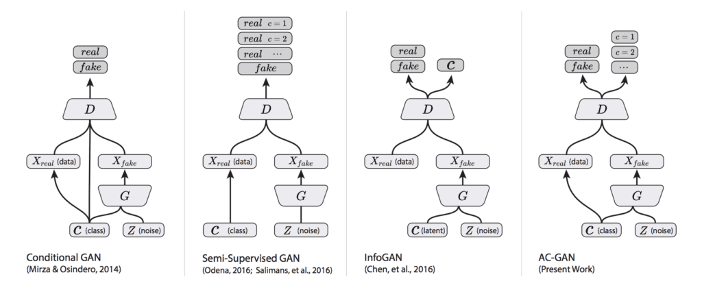
Summary of the Differences Between the Conditional GAN, Semi-Supervised GAN, InfoGAN, and AC-GAN.
Taken from: Version of Conditional Image Synthesis With Auxiliary Classifier GANs.
The discriminator seeks to maximize the probability of correctly classifying real and fake images (LS) and correctly predicting the class label (LC) of a real or fake image (e.g. LS + LC). The generator seeks to minimize the ability of the discriminator to discriminate real and fake images whilst also maximizing the ability of the discriminator predicting the class label of real and fake images (e.g. LC – LS).
The objective function has two parts: the log-likelihood of the correct source, LS, and the log-likelihood of the correct class, LC. […] D is trained to maximize LS + LC while G is trained to maximize LC − LS.
— Conditional Image Synthesis With Auxiliary Classifier GANs, 2016.
The resulting generator learns a latent space representation that is independent of the class label, unlike the conditional GAN.
AC-GANs learn a representation for z that is independent of class label.
— Conditional Image Synthesis With Auxiliary Classifier GANs, 2016.
The effect of changing the conditional GAN in this way is both a more stable training process and the ability of the model to generate higher quality images with a larger size than had been previously possible, e.g. 128×128 pixels.
… we demonstrate that adding more structure to the GAN latent space along with a specialized cost function results in higher quality samples. […] Importantly, we demonstrate quantitatively that our high resolution samples are not just naive resizings of low resolution samples.
— Conditional Image Synthesis With Auxiliary Classifier GANs, 2016.
Want to Develop GANs from Scratch?
Take my free 7-day email crash course now (with sample code).
Click to sign-up and also get a free PDF Ebook version of the course.
Fashion-MNIST Clothing Photograph Dataset
The Fashion-MNIST dataset is proposed as a more challenging replacement dataset for the MNIST handwritten digit dataset.
It is a dataset comprised of 60,000 small square 28×28 pixel grayscale images of items of 10 types of clothing, such as shoes, t-shirts, dresses, and more.
Keras provides access to the Fashion-MNIST dataset via the fashion_mnist.load_dataset() function. It returns two tuples, one with the input and output elements for the standard training dataset, and another with the input and output elements for the standard test dataset.
The example below loads the dataset and summarizes the shape of the loaded dataset.
Note: the first time you load the dataset, Keras will automatically download a compressed version of the images and save them under your home directory in ~/.keras/datasets/. The download is fast as the dataset is only about 25 megabytes in its compressed form.
# example of loading the fashion_mnist dataset
from keras.datasets.fashion_mnist import load_data
# load the images into memory
(trainX, trainy), (testX, testy) = load_data()
# summarize the shape of the dataset
print('Train', trainX.shape, trainy.shape)
print('Test', testX.shape, testy.shape)
Running the example loads the dataset and prints the shape of the input and output components of the train and test splits of images.
We can see that there are 60K examples in the training set and 10K in the test set and that each image is a square of 28 by 28 pixels.
Train (60000, 28, 28) (60000,)
Test (10000, 28, 28) (10000,)
The images are grayscale with a black background (0 pixel value) and the items of clothing in white ( pixel values near 255). This means if the images were plotted, they would be mostly black with a white item of clothing in the middle.
We can plot some of the images from the training dataset using the matplotlib library with the imshow() function and specify the color map via the ‘cmap‘ argument as ‘gray‘ to show the pixel values correctly.
# plot raw pixel data
pyplot.imshow(trainX[i], cmap='gray')
Alternately, the images are easier to review when we reverse the colors and plot the background as white and the clothing in black.
They are easier to view as most of the image is now white with the area of interest in black. This can be achieved using a reverse grayscale color map, as follows:
# plot raw pixel data
pyplot.imshow(trainX[i], cmap='gray_r')
The example below plots the first 100 images from the training dataset in a 10 by 10 square.
# example of loading the fashion_mnist dataset
from keras.datasets.fashion_mnist import load_data
from matplotlib import pyplot
# load the images into memory
(trainX, trainy), (testX, testy) = load_data()
# plot images from the training dataset
for i in range(100):
	# define subplot
	pyplot.subplot(10, 10, 1 + i)
	# turn off axis
	pyplot.axis('off')
	# plot raw pixel data
	pyplot.imshow(trainX[i], cmap='gray_r')
pyplot.show()
Running the example creates a figure with a plot of 100 images from the MNIST training dataset, arranged in a 10×10 square.
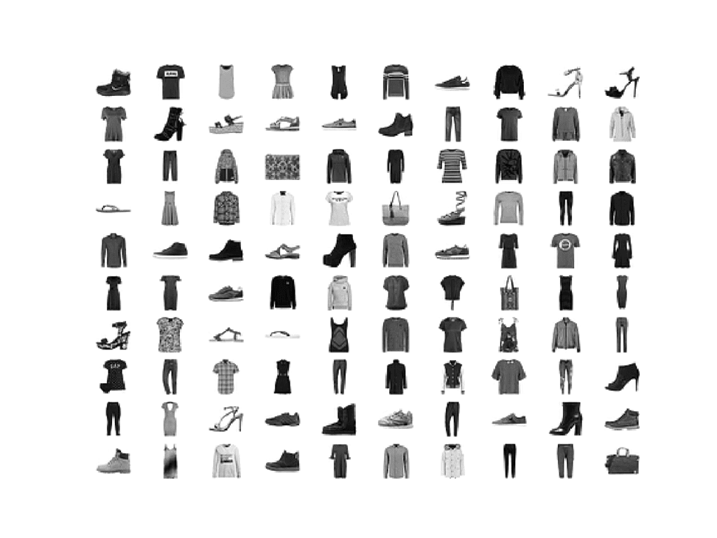
Plot of the First 100 Items of Clothing From the Fashion MNIST Dataset.
We will use the images in the training dataset as the basis for training a Generative Adversarial Network.
Specifically, the generator model will learn how to generate new plausible items of clothing, using a discriminator that will try to distinguish between real images from the Fashion MNIST training dataset and new images output by the generator model, and predict the class label for each.
This is a relatively simple problem that does not require a sophisticated generator or discriminator model, although it does require the generation of a grayscale output image.
How to Define AC-GAN Models
In this section, we will develop the generator, discriminator, and composite models for the AC-GAN.
The appendix of the AC-GAN paper provides suggestions for generator and discriminator configurations that we will use as inspiration. The table below summarizes these suggestions for the CIFAR-10 dataset, taken from the paper.
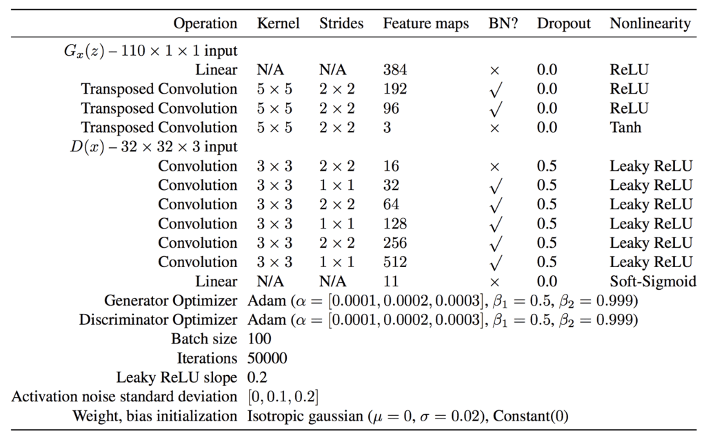
AC-GAN Generator and Discriminator Model Configuration Suggestions.
Take from: Conditional Image Synthesis With Auxiliary Classifier GANs.
AC-GAN Discriminator Model
Let’s start with the discriminator model.
The discriminator model must take as input an image and predict both the probability of the ‘realness‘ of the image and the probability of the image belonging to each of the given classes.
The input images will have the shape 28x28x1 and there are 10 classes for the items of clothing in the Fashion MNIST dataset.
The model can be defined as per the DCGAN architecture. That is, using Gaussian weight initialization, batch normalization, LeakyReLU, Dropout, and a 2×2 stride for downsampling instead of pooling layers.
For example, below is the bulk of the discriminator model defined using the Keras functional API.
...
# weight initialization
init = RandomNormal(stddev=0.02)
# image input
in_image = Input(shape=in_shape)
# downsample to 14x14
fe = Conv2D(32, (3,3), strides=(2,2), padding='same', kernel_initializer=init)(in_image)
fe = LeakyReLU(alpha=0.2)(fe)
fe = Dropout(0.5)(fe)
# normal
fe = Conv2D(64, (3,3), padding='same', kernel_initializer=init)(fe)
fe = BatchNormalization()(fe)
fe = LeakyReLU(alpha=0.2)(fe)
fe = Dropout(0.5)(fe)
# downsample to 7x7
fe = Conv2D(128, (3,3), strides=(2,2), padding='same', kernel_initializer=init)(fe)
fe = BatchNormalization()(fe)
fe = LeakyReLU(alpha=0.2)(fe)
fe = Dropout(0.5)(fe)
# normal
fe = Conv2D(256, (3,3), padding='same', kernel_initializer=init)(fe)
fe = BatchNormalization()(fe)
fe = LeakyReLU(alpha=0.2)(fe)
fe = Dropout(0.5)(fe)
# flatten feature maps
fe = Flatten()(fe)
...
The main difference is that the model has two output layers.
The first is a single node with the sigmoid activation for predicting the real-ness of the image.
...
# real/fake output
out1 = Dense(1, activation='sigmoid')(fe)
The second is multiple nodes, one for each class, using the softmax activation function to predict the class label of the given image.
...
# class label output
out2 = Dense(n_classes, activation='softmax')(fe)
We can then construct the image with a single input and two outputs.
...
# define model
model = Model(in_image, [out1, out2])
The model must be trained with two loss functions, binary cross entropy for the first output layer, and categorical cross-entropy loss for the second output layer.
Rather than comparing a one hot encoding of the class labels to the second output layer, as we might do normally, we can compare the integer class labels directly. We can achieve this automatically using the sparse categorical cross-entropy loss function. This will have the identical effect of the categorical cross-entropy but avoids the step of having to manually one hot encode the target labels.
When compiling the model, we can inform Keras to use the two different loss functions for the two output layers by specifying a list of function names as strings; for example:
loss=['binary_crossentropy', 'sparse_categorical_crossentropy']
The model is fit using the Adam version of stochastic gradient descent with a small learning rate and modest momentum, as is recommended for DCGANs.
...
# compile model
opt = Adam(lr=0.0002, beta_1=0.5)
model.compile(loss=['binary_crossentropy', 'sparse_categorical_crossentropy'], optimizer=opt)
Tying this together, the define_discriminator() function will define and compile the discriminator model for the AC-GAN.
The shape of the input images and the number of classes are parameterized and set with defaults, allowing them to be easily changed for your own project in the future.
# define the standalone discriminator model
def define_discriminator(in_shape=(28,28,1), n_classes=10):
	# weight initialization
	init = RandomNormal(stddev=0.02)
	# image input
	in_image = Input(shape=in_shape)
	# downsample to 14x14
	fe = Conv2D(32, (3,3), strides=(2,2), padding='same', kernel_initializer=init)(in_image)
	fe = LeakyReLU(alpha=0.2)(fe)
	fe = Dropout(0.5)(fe)
	# normal
	fe = Conv2D(64, (3,3), padding='same', kernel_initializer=init)(fe)
	fe = BatchNormalization()(fe)
	fe = LeakyReLU(alpha=0.2)(fe)
	fe = Dropout(0.5)(fe)
	# downsample to 7x7
	fe = Conv2D(128, (3,3), strides=(2,2), padding='same', kernel_initializer=init)(fe)
	fe = BatchNormalization()(fe)
	fe = LeakyReLU(alpha=0.2)(fe)
	fe = Dropout(0.5)(fe)
	# normal
	fe = Conv2D(256, (3,3), padding='same', kernel_initializer=init)(fe)
	fe = BatchNormalization()(fe)
	fe = LeakyReLU(alpha=0.2)(fe)
	fe = Dropout(0.5)(fe)
	# flatten feature maps
	fe = Flatten()(fe)
	# real/fake output
	out1 = Dense(1, activation='sigmoid')(fe)
	# class label output
	out2 = Dense(n_classes, activation='softmax')(fe)
	# define model
	model = Model(in_image, [out1, out2])
	# compile model
	opt = Adam(lr=0.0002, beta_1=0.5)
	model.compile(loss=['binary_crossentropy', 'sparse_categorical_crossentropy'], optimizer=opt)
	return model
We can define and summarize this model.
The complete example is listed below.
# example of defining the discriminator model
from keras.models import Model
from keras.layers import Input
from keras.layers import Dense
from keras.layers import Conv2D
from keras.layers import LeakyReLU
from keras.layers import Dropout
from keras.layers import Flatten
from keras.layers import BatchNormalization
from keras.initializers import RandomNormal
from keras.optimizers import Adam
from keras.utils.vis_utils import plot_model

# define the standalone discriminator model
def define_discriminator(in_shape=(28,28,1), n_classes=10):
	# weight initialization
	init = RandomNormal(stddev=0.02)
	# image input
	in_image = Input(shape=in_shape)
	# downsample to 14x14
	fe = Conv2D(32, (3,3), strides=(2,2), padding='same', kernel_initializer=init)(in_image)
	fe = LeakyReLU(alpha=0.2)(fe)
	fe = Dropout(0.5)(fe)
	# normal
	fe = Conv2D(64, (3,3), padding='same', kernel_initializer=init)(fe)
	fe = BatchNormalization()(fe)
	fe = LeakyReLU(alpha=0.2)(fe)
	fe = Dropout(0.5)(fe)
	# downsample to 7x7
	fe = Conv2D(128, (3,3), strides=(2,2), padding='same', kernel_initializer=init)(fe)
	fe = BatchNormalization()(fe)
	fe = LeakyReLU(alpha=0.2)(fe)
	fe = Dropout(0.5)(fe)
	# normal
	fe = Conv2D(256, (3,3), padding='same', kernel_initializer=init)(fe)
	fe = BatchNormalization()(fe)
	fe = LeakyReLU(alpha=0.2)(fe)
	fe = Dropout(0.5)(fe)
	# flatten feature maps
	fe = Flatten()(fe)
	# real/fake output
	out1 = Dense(1, activation='sigmoid')(fe)
	# class label output
	out2 = Dense(n_classes, activation='softmax')(fe)
	# define model
	model = Model(in_image, [out1, out2])
	# compile model
	opt = Adam(lr=0.0002, beta_1=0.5)
	model.compile(loss=['binary_crossentropy', 'sparse_categorical_crossentropy'], optimizer=opt)
	return model

# define the discriminator model
model = define_discriminator()
# summarize the model
model.summary()
# plot the model
plot_model(model, to_file='discriminator_plot.png', show_shapes=True, show_layer_names=True)
Running the example first prints a summary of the model.
This confirms the expected shape of the input images and the two output layers, although the linear organization does make the two separate output layers clear.
__________________________________________________________________________________________________
Layer (type)                    Output Shape         Param #     Connected to
==================================================================================================
input_1 (InputLayer)            (None, 28, 28, 1)    0
__________________________________________________________________________________________________
conv2d_1 (Conv2D)               (None, 14, 14, 32)   320         input_1[0][0]
__________________________________________________________________________________________________
leaky_re_lu_1 (LeakyReLU)       (None, 14, 14, 32)   0           conv2d_1[0][0]
__________________________________________________________________________________________________
dropout_1 (Dropout)             (None, 14, 14, 32)   0           leaky_re_lu_1[0][0]
__________________________________________________________________________________________________
conv2d_2 (Conv2D)               (None, 14, 14, 64)   18496       dropout_1[0][0]
__________________________________________________________________________________________________
batch_normalization_1 (BatchNor (None, 14, 14, 64)   256         conv2d_2[0][0]
__________________________________________________________________________________________________
leaky_re_lu_2 (LeakyReLU)       (None, 14, 14, 64)   0           batch_normalization_1[0][0]
__________________________________________________________________________________________________
dropout_2 (Dropout)             (None, 14, 14, 64)   0           leaky_re_lu_2[0][0]
__________________________________________________________________________________________________
conv2d_3 (Conv2D)               (None, 7, 7, 128)    73856       dropout_2[0][0]
__________________________________________________________________________________________________
batch_normalization_2 (BatchNor (None, 7, 7, 128)    512         conv2d_3[0][0]
__________________________________________________________________________________________________
leaky_re_lu_3 (LeakyReLU)       (None, 7, 7, 128)    0           batch_normalization_2[0][0]
__________________________________________________________________________________________________
dropout_3 (Dropout)             (None, 7, 7, 128)    0           leaky_re_lu_3[0][0]
__________________________________________________________________________________________________
conv2d_4 (Conv2D)               (None, 7, 7, 256)    295168      dropout_3[0][0]
__________________________________________________________________________________________________
batch_normalization_3 (BatchNor (None, 7, 7, 256)    1024        conv2d_4[0][0]
__________________________________________________________________________________________________
leaky_re_lu_4 (LeakyReLU)       (None, 7, 7, 256)    0           batch_normalization_3[0][0]
__________________________________________________________________________________________________
dropout_4 (Dropout)             (None, 7, 7, 256)    0           leaky_re_lu_4[0][0]
__________________________________________________________________________________________________
flatten_1 (Flatten)             (None, 12544)        0           dropout_4[0][0]
__________________________________________________________________________________________________
dense_1 (Dense)                 (None, 1)            12545       flatten_1[0][0]
__________________________________________________________________________________________________
dense_2 (Dense)                 (None, 10)           125450      flatten_1[0][0]
==================================================================================================
Total params: 527,627
Trainable params: 526,731
Non-trainable params: 896
__________________________________________________________________________________________________
A plot of the model is also created, showing the linear processing of the input image and the two clear output layers.
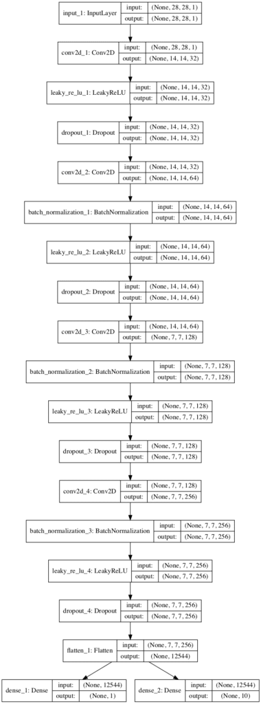
Plot of the Discriminator Model for the Auxiliary Classifier GAN
Now that we have defined our AC-GAN discriminator model, we can develop the generator model.
AC-GAN Generator Model
The generator model must take a random point from the latent space as input, and the class label, then output a generated grayscale image with the shape 28x28x1.
The AC-GAN paper describes the AC-GAN generator model taking a vector input that is a concatenation of the point in latent space (100 dimensions) and the one hot encoded class label (10 dimensions) that is 110 dimensions.
An alternative approach that has proven effective and is now generally recommended is to interpret the class label as an additional channel or feature map early in the generator model.
This can be achieved by using a learned embedding with an arbitrary number of dimensions (e.g. 50), the output of which can be interpreted by a fully connected layer with a linear activation resulting in one additional 7×7 feature map.
...
# label input
in_label = Input(shape=(1,))
# embedding for categorical input
li = Embedding(n_classes, 50)(in_label)
# linear multiplication
n_nodes = 7 * 7
li = Dense(n_nodes, kernel_initializer=init)(li)
# reshape to additional channel
li = Reshape((7, 7, 1))(li)
The point in latent space can be interpreted by a fully connected layer with sufficient activations to create multiple 7×7 feature maps, in this case, 384, and provide the basis for a low-resolution version of our output image.
The 7×7 single feature map interpretation of the class label can then be channel-wise concatenated, resulting in 385 feature maps.
...
# image generator input
in_lat = Input(shape=(latent_dim,))
# foundation for 7x7 image
n_nodes = 384 * 7 * 7
gen = Dense(n_nodes, kernel_initializer=init)(in_lat)
gen = Activation('relu')(gen)
gen = Reshape((7, 7, 384))(gen)
# merge image gen and label input
merge = Concatenate()([gen, li])
These feature maps can then go through the process of two transpose convolutional layers to upsample the 7×7 feature maps first to 14×14 pixels, and then finally to 28×28 features, quadrupling the area of the feature maps with each upscaling step.
The output of the generator is a single feature map or grayscale image with the shape 28×28 and pixel values in the range [-1, 1] given the choice of a tanh activation function. We use ReLU activation for the upscaling layers instead of LeakyReLU given the suggestion the AC-GAN paper.
# upsample to 14x14
gen = Conv2DTranspose(192, (5,5), strides=(2,2), padding='same', kernel_initializer=init)(merge)
gen = BatchNormalization()(gen)
gen = Activation('relu')(gen)
# upsample to 28x28
gen = Conv2DTranspose(1, (5,5), strides=(2,2), padding='same', kernel_initializer=init)(gen)
out_layer = Activation('tanh')(gen)
We can tie all of this together and into the define_generator() function defined below that will create and return the generator model for the AC-GAN.
The model is intentionally not compiled as it is not trained directly; instead, it is trained via the discriminator model.
# define the standalone generator model
def define_generator(latent_dim, n_classes=10):
	# weight initialization
	init = RandomNormal(stddev=0.02)
	# label input
	in_label = Input(shape=(1,))
	# embedding for categorical input
	li = Embedding(n_classes, 50)(in_label)
	# linear multiplication
	n_nodes = 7 * 7
	li = Dense(n_nodes, kernel_initializer=init)(li)
	# reshape to additional channel
	li = Reshape((7, 7, 1))(li)
	# image generator input
	in_lat = Input(shape=(latent_dim,))
	# foundation for 7x7 image
	n_nodes = 384 * 7 * 7
	gen = Dense(n_nodes, kernel_initializer=init)(in_lat)
	gen = Activation('relu')(gen)
	gen = Reshape((7, 7, 384))(gen)
	# merge image gen and label input
	merge = Concatenate()([gen, li])
	# upsample to 14x14
	gen = Conv2DTranspose(192, (5,5), strides=(2,2), padding='same', kernel_initializer=init)(merge)
	gen = BatchNormalization()(gen)
	gen = Activation('relu')(gen)
	# upsample to 28x28
	gen = Conv2DTranspose(1, (5,5), strides=(2,2), padding='same', kernel_initializer=init)(gen)
	out_layer = Activation('tanh')(gen)
	# define model
	model = Model([in_lat, in_label], out_layer)
	return model
We can create this model and summarize and plot its structure.
The complete example is listed below.
# example of defining the generator model
from keras.models import Model
from keras.layers import Input
from keras.layers import Dense
from keras.layers import Reshape
from keras.layers import Conv2DTranspose
from keras.layers import Embedding
from keras.layers import Concatenate
from keras.layers import Activation
from keras.layers import BatchNormalization
from keras.initializers import RandomNormal
from keras.utils.vis_utils import plot_model

# define the standalone generator model
def define_generator(latent_dim, n_classes=10):
	# weight initialization
	init = RandomNormal(stddev=0.02)
	# label input
	in_label = Input(shape=(1,))
	# embedding for categorical input
	li = Embedding(n_classes, 50)(in_label)
	# linear multiplication
	n_nodes = 7 * 7
	li = Dense(n_nodes, kernel_initializer=init)(li)
	# reshape to additional channel
	li = Reshape((7, 7, 1))(li)
	# image generator input
	in_lat = Input(shape=(latent_dim,))
	# foundation for 7x7 image
	n_nodes = 384 * 7 * 7
	gen = Dense(n_nodes, kernel_initializer=init)(in_lat)
	gen = Activation('relu')(gen)
	gen = Reshape((7, 7, 384))(gen)
	# merge image gen and label input
	merge = Concatenate()([gen, li])
	# upsample to 14x14
	gen = Conv2DTranspose(192, (5,5), strides=(2,2), padding='same', kernel_initializer=init)(merge)
	gen = BatchNormalization()(gen)
	gen = Activation('relu')(gen)
	# upsample to 28x28
	gen = Conv2DTranspose(1, (5,5), strides=(2,2), padding='same', kernel_initializer=init)(gen)
	out_layer = Activation('tanh')(gen)
	# define model
	model = Model([in_lat, in_label], out_layer)
	return model

# define the size of the latent space
latent_dim = 100
# define the generator model
model = define_generator(latent_dim)
# summarize the model
model.summary()
# plot the model
plot_model(model, to_file='generator_plot.png', show_shapes=True, show_layer_names=True)
Running the example first prints a summary of the layers and their output shape in the model.
We can confirm that the latent dimension input is 100 dimensions and that the class label input is a single integer. We can also confirm that the output of the embedding class label is correctly concatenated as an additional channel resulting in 385 7×7 feature maps prior to the transpose convolutional layers.
The summary also confirms the expected output shape of a single grayscale 28×28 image.
__________________________________________________________________________________________________
Layer (type)                    Output Shape         Param #     Connected to
==================================================================================================
input_2 (InputLayer)            (None, 100)          0
__________________________________________________________________________________________________
input_1 (InputLayer)            (None, 1)            0
__________________________________________________________________________________________________
dense_2 (Dense)                 (None, 18816)        1900416     input_2[0][0]
__________________________________________________________________________________________________
embedding_1 (Embedding)         (None, 1, 50)        500         input_1[0][0]
__________________________________________________________________________________________________
activation_1 (Activation)       (None, 18816)        0           dense_2[0][0]
__________________________________________________________________________________________________
dense_1 (Dense)                 (None, 1, 49)        2499        embedding_1[0][0]
__________________________________________________________________________________________________
reshape_2 (Reshape)             (None, 7, 7, 384)    0           activation_1[0][0]
__________________________________________________________________________________________________
reshape_1 (Reshape)             (None, 7, 7, 1)      0           dense_1[0][0]
__________________________________________________________________________________________________
concatenate_1 (Concatenate)     (None, 7, 7, 385)    0           reshape_2[0][0]
                                                                 reshape_1[0][0]
__________________________________________________________________________________________________
conv2d_transpose_1 (Conv2DTrans (None, 14, 14, 192)  1848192     concatenate_1[0][0]
__________________________________________________________________________________________________
batch_normalization_1 (BatchNor (None, 14, 14, 192)  768         conv2d_transpose_1[0][0]
__________________________________________________________________________________________________
activation_2 (Activation)       (None, 14, 14, 192)  0           batch_normalization_1[0][0]
__________________________________________________________________________________________________
conv2d_transpose_2 (Conv2DTrans (None, 28, 28, 1)    4801        activation_2[0][0]
__________________________________________________________________________________________________
activation_3 (Activation)       (None, 28, 28, 1)    0           conv2d_transpose_2[0][0]
==================================================================================================
Total params: 3,757,176
Trainable params: 3,756,792
Non-trainable params: 384
__________________________________________________________________________________________________
A plot of the network is also created summarizing the input and output shapes for each layer.
The plot confirms the two inputs to the network and the correct concatenation of the inputs.
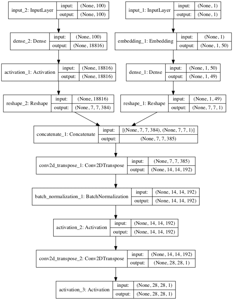
Plot of the Generator Model for the Auxiliary Classifier GAN
Now that we have defined the generator model, we can show how it might be fit.
AC-GAN Composite Model
The generator model is not updated directly; instead, it is updated via the discriminator model.
This can be achieved by creating a composite model that stacks the generator model on top of the discriminator model.
The input to this composite model is the input to the generator model, namely a random point from the latent space and a class label. The generator model is connected directly to the discriminator model, which takes the generated image directly as input. Finally, the discriminator model predicts both the realness of the generated image and the class label. As such, the composite model is optimized using two loss functions, one for each output of the discriminator model.
The discriminator model is updated in a standalone manner using real and fake examples, and we will review how to do this in the next section. Therefore, we do not want to update the discriminator model when updating (training) the composite model; we only want to use this composite model to update the weights of the generator model.
This can be achieved by setting the layers of the discriminator as not trainable prior to compiling the composite model. This only has an effect on the layer weights when viewed or used by the composite model and prevents them from being updated when the composite model is updated.
The define_gan() function below implements this, taking the already defined generator and discriminator models as input and defining a new composite model that can be used to update the generator model only.
# define the combined generator and discriminator model, for updating the generator
def define_gan(g_model, d_model):
	# make weights in the discriminator not trainable
	d_model.trainable = False
	# connect the outputs of the generator to the inputs of the discriminator
	gan_output = d_model(g_model.output)
	# define gan model as taking noise and label and outputting real/fake and label outputs
	model = Model(g_model.input, gan_output)
	# compile model
	opt = Adam(lr=0.0002, beta_1=0.5)
	model.compile(loss=['binary_crossentropy', 'sparse_categorical_crossentropy'], optimizer=opt)
	return model
Now that we have defined the models used in the AC-GAN, we can fit them on the Fashion-MNIST dataset.
How to Develop an AC-GAN for Fashion-MNIST
The first step is to load and prepare the Fashion MNIST dataset.
We only require the images in the training dataset. The images are black and white, therefore we must add an additional channel dimension to transform them to be three dimensional, as expected by the convolutional layers of our models. Finally, the pixel values must be scaled to the range [-1,1] to match the output of the generator model.
The load_real_samples() function below implements this, returning the loaded and scaled Fashion MNIST training dataset ready for modeling.
# load images
def load_real_samples():
	# load dataset
	(trainX, trainy), (_, _) = load_data()
	# expand to 3d, e.g. add channels
	X = expand_dims(trainX, axis=-1)
	# convert from ints to floats
	X = X.astype('float32')
	# scale from [0,255] to [-1,1]
	X = (X - 127.5) / 127.5
	print(X.shape, trainy.shape)
	return [X, trainy]
We will require one batch (or a half batch) of real images from the dataset each update to the GAN model. A simple way to achieve this is to select a random sample of images from the dataset each time.
The generate_real_samples() function below implements this, taking the prepared dataset as an argument, selecting and returning a random sample of Fashion MNIST images and clothing class labels.
The “dataset” argument provided to the function is a list comprised of the images and class labels as returned from the load_real_samples() function. The function also returns their corresponding class label for the discriminator, specifically class=1 indicating that they are real images.
# select real samples
def generate_real_samples(dataset, n_samples):
	# split into images and labels
	images, labels = dataset
	# choose random instances
	ix = randint(0, images.shape[0], n_samples)
	# select images and labels
	X, labels = images[ix], labels[ix]
	# generate class labels
	y = ones((n_samples, 1))
	return [X, labels], y
Next, we need inputs for the generator model.
These are random points from the latent space, specifically Gaussian distributed random variables.
The generate_latent_points() function implements this, taking the size of the latent space as an argument and the number of points required, and returning them as a batch of input samples for the generator model. The function also returns randomly selected integers in [0,9] inclusively for the 10 class labels in the Fashion-MNIST dataset.
# generate points in latent space as input for the generator
def generate_latent_points(latent_dim, n_samples, n_classes=10):
	# generate points in the latent space
	x_input = randn(latent_dim * n_samples)
	# reshape into a batch of inputs for the network
	z_input = x_input.reshape(n_samples, latent_dim)
	# generate labels
	labels = randint(0, n_classes, n_samples)
	return [z_input, labels]
Next, we need to use the points in the latent space and clothing class labels as input to the generator in order to generate new images.
The generate_fake_samples() function below implements this, taking the generator model and size of the latent space as arguments, then generating points in the latent space and using them as input to the generator model.
The function returns the generated images, their corresponding clothing class label, and their discriminator class label, specifically class=0 to indicate they are fake or generated.
# use the generator to generate n fake examples, with class labels
def generate_fake_samples(generator, latent_dim, n_samples):
	# generate points in latent space
	z_input, labels_input = generate_latent_points(latent_dim, n_samples)
	# predict outputs
	images = generator.predict([z_input, labels_input])
	# create class labels
	y = zeros((n_samples, 1))
	return [images, labels_input], y
There are no reliable ways to determine when to stop training a GAN; instead, images can be subjectively inspected in order to choose a final model.
Therefore, we can periodically generate a sample of images using the generator model and save the generator model to file for later use. The summarize_performance() function below implements this, generating 100 images, plotting them, and saving the plot and the generator to file with a filename that includes the training “step” number.
# generate samples and save as a plot and save the model
def summarize_performance(step, g_model, latent_dim, n_samples=100):
	# prepare fake examples
	[X, _], _ = generate_fake_samples(g_model, latent_dim, n_samples)
	# scale from [-1,1] to [0,1]
	X = (X + 1) / 2.0
	# plot images
	for i in range(100):
		# define subplot
		pyplot.subplot(10, 10, 1 + i)
		# turn off axis
		pyplot.axis('off')
		# plot raw pixel data
		pyplot.imshow(X[i, :, :, 0], cmap='gray_r')
	# save plot to file
	filename1 = 'generated_plot_%04d.png' % (step+1)
	pyplot.savefig(filename1)
	pyplot.close()
	# save the generator model
	filename2 = 'model_%04d.h5' % (step+1)
	g_model.save(filename2)
	print('>Saved: %s and %s' % (filename1, filename2))
We are now ready to fit the GAN models.
The model is fit for 100 training epochs, which is arbitrary, as the model begins generating plausible items of clothing after perhaps 20 epochs. A batch size of 64 samples is used, and each training epoch involves 60,000/64, or about 937, batches of real and fake samples and updates to the model. The summarize_performance() function is called every 10 epochs, or every (937 * 10) 9,370 training steps.
For a given training step, first the discriminator model is updated for a half batch of real samples, then a half batch of fake samples, together forming one batch of weight updates. The generator is then updated via the combined GAN model. Importantly, the class label is set to 1, or real, for the fake samples. This has the effect of updating the generator toward getting better at generating real samples on the next batch.
Note, the discriminator and composite model return three loss values from the call to the train_on_batch() function. The first value is the sum of the loss values and can be ignored, whereas the second value is the loss for the real/fake output layer and the third value is the loss for the clothing label classification.
The train() function below implements this, taking the defined models, dataset, and size of the latent dimension as arguments and parameterizing the number of epochs and batch size with default arguments. The generator model is saved at the end of training.
# train the generator and discriminator
def train(g_model, d_model, gan_model, dataset, latent_dim, n_epochs=100, n_batch=64):
	# calculate the number of batches per training epoch
	bat_per_epo = int(dataset[0].shape[0] / n_batch)
	# calculate the number of training iterations
	n_steps = bat_per_epo * n_epochs
	# calculate the size of half a batch of samples
	half_batch = int(n_batch / 2)
	# manually enumerate epochs
	for i in range(n_steps):
		# get randomly selected 'real' samples
		[X_real, labels_real], y_real = generate_real_samples(dataset, half_batch)
		# update discriminator model weights
		_,d_r1,d_r2 = d_model.train_on_batch(X_real, [y_real, labels_real])
		# generate 'fake' examples
		[X_fake, labels_fake], y_fake = generate_fake_samples(g_model, latent_dim, half_batch)
		# update discriminator model weights
		_,d_f,d_f2 = d_model.train_on_batch(X_fake, [y_fake, labels_fake])
		# prepare points in latent space as input for the generator
		[z_input, z_labels] = generate_latent_points(latent_dim, n_batch)
		# create inverted labels for the fake samples
		y_gan = ones((n_batch, 1))
		# update the generator via the discriminator's error
		_,g_1,g_2 = gan_model.train_on_batch([z_input, z_labels], [y_gan, z_labels])
		# summarize loss on this batch
		print('>%d, dr[%.3f,%.3f], df[%.3f,%.3f], g[%.3f,%.3f]' % (i+1, d_r1,d_r2, d_f,d_f2, g_1,g_2))
		# evaluate the model performance every 'epoch'
		if (i+1) % (bat_per_epo * 10) == 0:
			summarize_performance(i, g_model, latent_dim)
We can then define the size of the latent space, define all three models, and train them on the loaded fashion MNIST dataset.
# size of the latent space
latent_dim = 100
# create the discriminator
discriminator = define_discriminator()
# create the generator
generator = define_generator(latent_dim)
# create the gan
gan_model = define_gan(generator, discriminator)
# load image data
dataset = load_real_samples()
# train model
train(generator, discriminator, gan_model, dataset, latent_dim)
Tying all of this together, the complete example is listed below.
# example of fitting an auxiliary classifier gan (ac-gan) on fashion mnsit
from numpy import zeros
from numpy import ones
from numpy import expand_dims
from numpy.random import randn
from numpy.random import randint
from keras.datasets.fashion_mnist import load_data
from keras.optimizers import Adam
from keras.models import Model
from keras.layers import Input
from keras.layers import Dense
from keras.layers import Reshape
from keras.layers import Flatten
from keras.layers import Conv2D
from keras.layers import Conv2DTranspose
from keras.layers import LeakyReLU
from keras.layers import BatchNormalization
from keras.layers import Dropout
from keras.layers import Embedding
from keras.layers import Activation
from keras.layers import Concatenate
from keras.initializers import RandomNormal
from matplotlib import pyplot

# define the standalone discriminator model
def define_discriminator(in_shape=(28,28,1), n_classes=10):
	# weight initialization
	init = RandomNormal(stddev=0.02)
	# image input
	in_image = Input(shape=in_shape)
	# downsample to 14x14
	fe = Conv2D(32, (3,3), strides=(2,2), padding='same', kernel_initializer=init)(in_image)
	fe = LeakyReLU(alpha=0.2)(fe)
	fe = Dropout(0.5)(fe)
	# normal
	fe = Conv2D(64, (3,3), padding='same', kernel_initializer=init)(fe)
	fe = BatchNormalization()(fe)
	fe = LeakyReLU(alpha=0.2)(fe)
	fe = Dropout(0.5)(fe)
	# downsample to 7x7
	fe = Conv2D(128, (3,3), strides=(2,2), padding='same', kernel_initializer=init)(fe)
	fe = BatchNormalization()(fe)
	fe = LeakyReLU(alpha=0.2)(fe)
	fe = Dropout(0.5)(fe)
	# normal
	fe = Conv2D(256, (3,3), padding='same', kernel_initializer=init)(fe)
	fe = BatchNormalization()(fe)
	fe = LeakyReLU(alpha=0.2)(fe)
	fe = Dropout(0.5)(fe)
	# flatten feature maps
	fe = Flatten()(fe)
	# real/fake output
	out1 = Dense(1, activation='sigmoid')(fe)
	# class label output
	out2 = Dense(n_classes, activation='softmax')(fe)
	# define model
	model = Model(in_image, [out1, out2])
	# compile model
	opt = Adam(lr=0.0002, beta_1=0.5)
	model.compile(loss=['binary_crossentropy', 'sparse_categorical_crossentropy'], optimizer=opt)
	return model

# define the standalone generator model
def define_generator(latent_dim, n_classes=10):
	# weight initialization
	init = RandomNormal(stddev=0.02)
	# label input
	in_label = Input(shape=(1,))
	# embedding for categorical input
	li = Embedding(n_classes, 50)(in_label)
	# linear multiplication
	n_nodes = 7 * 7
	li = Dense(n_nodes, kernel_initializer=init)(li)
	# reshape to additional channel
	li = Reshape((7, 7, 1))(li)
	# image generator input
	in_lat = Input(shape=(latent_dim,))
	# foundation for 7x7 image
	n_nodes = 384 * 7 * 7
	gen = Dense(n_nodes, kernel_initializer=init)(in_lat)
	gen = Activation('relu')(gen)
	gen = Reshape((7, 7, 384))(gen)
	# merge image gen and label input
	merge = Concatenate()([gen, li])
	# upsample to 14x14
	gen = Conv2DTranspose(192, (5,5), strides=(2,2), padding='same', kernel_initializer=init)(merge)
	gen = BatchNormalization()(gen)
	gen = Activation('relu')(gen)
	# upsample to 28x28
	gen = Conv2DTranspose(1, (5,5), strides=(2,2), padding='same', kernel_initializer=init)(gen)
	out_layer = Activation('tanh')(gen)
	# define model
	model = Model([in_lat, in_label], out_layer)
	return model

# define the combined generator and discriminator model, for updating the generator
def define_gan(g_model, d_model):
	# make weights in the discriminator not trainable
	d_model.trainable = False
	# connect the outputs of the generator to the inputs of the discriminator
	gan_output = d_model(g_model.output)
	# define gan model as taking noise and label and outputting real/fake and label outputs
	model = Model(g_model.input, gan_output)
	# compile model
	opt = Adam(lr=0.0002, beta_1=0.5)
	model.compile(loss=['binary_crossentropy', 'sparse_categorical_crossentropy'], optimizer=opt)
	return model

# load images
def load_real_samples():
	# load dataset
	(trainX, trainy), (_, _) = load_data()
	# expand to 3d, e.g. add channels
	X = expand_dims(trainX, axis=-1)
	# convert from ints to floats
	X = X.astype('float32')
	# scale from [0,255] to [-1,1]
	X = (X - 127.5) / 127.5
	print(X.shape, trainy.shape)
	return [X, trainy]

# select real samples
def generate_real_samples(dataset, n_samples):
	# split into images and labels
	images, labels = dataset
	# choose random instances
	ix = randint(0, images.shape[0], n_samples)
	# select images and labels
	X, labels = images[ix], labels[ix]
	# generate class labels
	y = ones((n_samples, 1))
	return [X, labels], y

# generate points in latent space as input for the generator
def generate_latent_points(latent_dim, n_samples, n_classes=10):
	# generate points in the latent space
	x_input = randn(latent_dim * n_samples)
	# reshape into a batch of inputs for the network
	z_input = x_input.reshape(n_samples, latent_dim)
	# generate labels
	labels = randint(0, n_classes, n_samples)
	return [z_input, labels]

# use the generator to generate n fake examples, with class labels
def generate_fake_samples(generator, latent_dim, n_samples):
	# generate points in latent space
	z_input, labels_input = generate_latent_points(latent_dim, n_samples)
	# predict outputs
	images = generator.predict([z_input, labels_input])
	# create class labels
	y = zeros((n_samples, 1))
	return [images, labels_input], y

# generate samples and save as a plot and save the model
def summarize_performance(step, g_model, latent_dim, n_samples=100):
	# prepare fake examples
	[X, _], _ = generate_fake_samples(g_model, latent_dim, n_samples)
	# scale from [-1,1] to [0,1]
	X = (X + 1) / 2.0
	# plot images
	for i in range(100):
		# define subplot
		pyplot.subplot(10, 10, 1 + i)
		# turn off axis
		pyplot.axis('off')
		# plot raw pixel data
		pyplot.imshow(X[i, :, :, 0], cmap='gray_r')
	# save plot to file
	filename1 = 'generated_plot_%04d.png' % (step+1)
	pyplot.savefig(filename1)
	pyplot.close()
	# save the generator model
	filename2 = 'model_%04d.h5' % (step+1)
	g_model.save(filename2)
	print('>Saved: %s and %s' % (filename1, filename2))

# train the generator and discriminator
def train(g_model, d_model, gan_model, dataset, latent_dim, n_epochs=100, n_batch=64):
	# calculate the number of batches per training epoch
	bat_per_epo = int(dataset[0].shape[0] / n_batch)
	# calculate the number of training iterations
	n_steps = bat_per_epo * n_epochs
	# calculate the size of half a batch of samples
	half_batch = int(n_batch / 2)
	# manually enumerate epochs
	for i in range(n_steps):
		# get randomly selected 'real' samples
		[X_real, labels_real], y_real = generate_real_samples(dataset, half_batch)
		# update discriminator model weights
		_,d_r1,d_r2 = d_model.train_on_batch(X_real, [y_real, labels_real])
		# generate 'fake' examples
		[X_fake, labels_fake], y_fake = generate_fake_samples(g_model, latent_dim, half_batch)
		# update discriminator model weights
		_,d_f,d_f2 = d_model.train_on_batch(X_fake, [y_fake, labels_fake])
		# prepare points in latent space as input for the generator
		[z_input, z_labels] = generate_latent_points(latent_dim, n_batch)
		# create inverted labels for the fake samples
		y_gan = ones((n_batch, 1))
		# update the generator via the discriminator's error
		_,g_1,g_2 = gan_model.train_on_batch([z_input, z_labels], [y_gan, z_labels])
		# summarize loss on this batch
		print('>%d, dr[%.3f,%.3f], df[%.3f,%.3f], g[%.3f,%.3f]' % (i+1, d_r1,d_r2, d_f,d_f2, g_1,g_2))
		# evaluate the model performance every 'epoch'
		if (i+1) % (bat_per_epo * 10) == 0:
			summarize_performance(i, g_model, latent_dim)

# size of the latent space
latent_dim = 100
# create the discriminator
discriminator = define_discriminator()
# create the generator
generator = define_generator(latent_dim)
# create the gan
gan_model = define_gan(generator, discriminator)
# load image data
dataset = load_real_samples()
# train model
train(generator, discriminator, gan_model, dataset, latent_dim)
Running the example may take some time, and GPU hardware is recommended, but not required.
Note: Given the stochastic nature of the training algorithm, your results may vary. Try running the example a few times.
The loss is reported each training iteration, including the real/fake and class loss for the discriminator on real examples (dr), the discriminator on fake examples (df), and the generator updated via the composite model when generating images (g).
>1, dr[0.934,2.967], df[1.310,3.006], g[0.878,3.368]
>2, dr[0.711,2.836], df[0.939,3.262], g[0.947,2.751]
>3, dr[0.649,2.980], df[1.001,3.147], g[0.844,3.226]
>4, dr[0.732,3.435], df[0.823,3.715], g[1.048,3.292]
>5, dr[0.860,3.076], df[0.591,2.799], g[1.123,3.313]
...
A total of 10 sample images are generated and 10 models saved over the run.
Plots of generated clothing after 10 iterations already look plausible.

Example of AC-GAN Generated Items of Clothing after 10 Epochs
The images remain reliable throughout the training process.
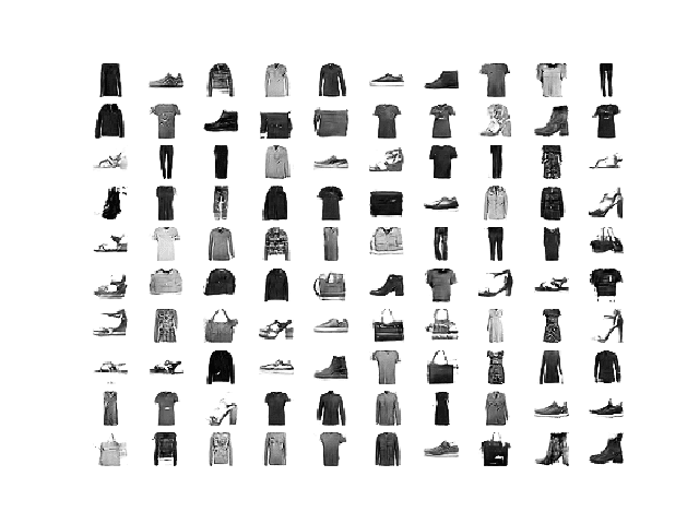
Example of AC-GAN Generated Items of Clothing After 100 Epochs
How to Generate Items of Clothing With the AC-GAN
In this section, we can load a saved model and use it to generate new items of clothing that plausibly could have come from the Fashion-MNIST dataset.
The AC-GAN technically does not conditionally generate images based on the class label, at least not in the same way as the conditional GAN.
AC-GANs learn a representation for z that is independent of class label.
— Conditional Image Synthesis With Auxiliary Classifier GANs, 2016.
Nevertheless, if used in this way, the generated images mostly match the class label.
The example below loads the model from the end of the run (any saved model would do), and generates 100 examples of class 7 (sneaker).
# example of loading the generator model and generating images
from math import sqrt
from numpy import asarray
from numpy.random import randn
from keras.models import load_model
from matplotlib import pyplot

# generate points in latent space as input for the generator
def generate_latent_points(latent_dim, n_samples, n_class):
	# generate points in the latent space
	x_input = randn(latent_dim * n_samples)
	# reshape into a batch of inputs for the network
	z_input = x_input.reshape(n_samples, latent_dim)
	# generate labels
	labels = asarray([n_class for _ in range(n_samples)])
	return [z_input, labels]

# create and save a plot of generated images
def save_plot(examples, n_examples):
	# plot images
	for i in range(n_examples):
		# define subplot
		pyplot.subplot(sqrt(n_examples), sqrt(n_examples), 1 + i)
		# turn off axis
		pyplot.axis('off')
		# plot raw pixel data
		pyplot.imshow(examples[i, :, :, 0], cmap='gray_r')
	pyplot.show()

# load model
model = load_model('model_93700.h5')
latent_dim = 100
n_examples = 100 # must be a square
n_class = 7 # sneaker
# generate images
latent_points, labels = generate_latent_points(latent_dim, n_examples, n_class)
# generate images
X  = model.predict([latent_points, labels])
# scale from [-1,1] to [0,1]
X = (X + 1) / 2.0
# plot the result
save_plot(X, n_examples)
Running the example, in this case, generates 100 very plausible photos of sneakers.
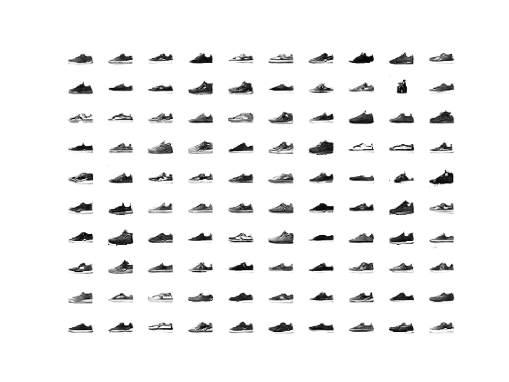
Example of 100 Photos of Sneakers Generated by an AC-GAN
It may be fun to experiment with other class values.
For example, below are 100 generated coats (n_class = 4). Most of the images are coats, although there are a few pants in there, showing that the latent space is partially, but not completely, class-conditional.
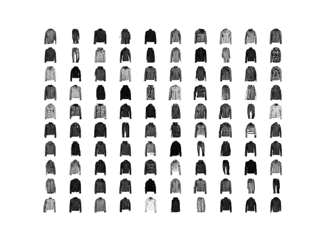
Example of 100 Photos of Coats Generated by an AC-GAN
Extensions
This section lists some ideas for extending the tutorial that you may wish to explore.
- Generate Images. Generate images for each clothing class and compare results across different saved models (e.g. epoch 10, 20, etc.).
- Alternate Configuration. Update the configuration of the generator, discriminator, or both models to have more or less capacity and compare results.
- CIFAR-10 Dataset. Update the example to train on the CIFAR-10 dataset and use model configuration described in the appendix of the paper.
If you explore any of these extensions, I’d love to know.
Post your findings in the comments below.
Further Reading
This section provides more resources on the topic if you are looking to go deeper.
Papers
- Conditional Image Synthesis With Auxiliary Classifier GANs, 2016.
- Conditional Image Synthesis With Auxiliary Classifier GANs, Reviewer Comments.
- Conditional Image Synthesis with Auxiliary Classifier GANs, NIPS 2016, YouTube.
API
- Keras Datasets API.
- Keras Sequential Model API
- Keras Convolutional Layers API
- How can I “freeze” Keras layers?
- MatplotLib API
- NumPy Random sampling (numpy.random) API
- NumPy Array manipulation routines
Articles
- How to Train a GAN? Tips and tricks to make GANs work
- Fashion-MNIST Project, GitHub.
- AC-GAN, Keras GAN Project.
- AC-GAN, Keras Example.
Summary
In this tutorial, you discovered how to develop an auxiliary classifier generative adversarial network for generating photographs of clothing.
Specifically, you learned:
- The auxiliary classifier GAN is a type of conditional GAN that requires that the discriminator predict the class label of a given image.
- How to develop generator, discriminator, and composite models for the AC-GAN.
- How to train, evaluate, and use an AC-GAN to generate photographs of clothing from the Fashion-MNIST dataset.
Do you have any questions?
Ask your questions in the comments below and I will do my best to answer.
The post How to Develop an Auxiliary Classifier GAN (AC-GAN) From Scratch with Keras appeared first on Machine Learning Mastery.
