
Author: Jason Brownlee
Machine learning predictive modeling performance is only as good as your data, and your data is only as good as the way you prepare it for modeling.
The most common approach to data preparation is to study a dataset and review the expectations of a machine learning algorithms, then carefully choose the most appropriate data preparation techniques to transform the raw data to best meet the expectations of the algorithm. This is slow, expensive, and requires a vast amount of expertise.
An alternative approach to data preparation is to grid search a suite of common and commonly useful data preparation techniques to the raw data. This is an alternative philosophy for data preparation that treats data transforms as another hyperparameter of the modeling pipeline to be searched and tuned.
This approach requires less expertise than the traditional manual approach to data preparation, although it is computationally costly. The benefit is that it can aid in the discovery of non-intuitive data preparation solutions that achieve good or best performance for a given predictive modeling problem.
In this tutorial, you will discover how to use the grid search approach for data preparation with tabular data.
After completing this tutorial, you will know:
- Grid search provides an alternative approach to data preparation for tabular data, where transforms are tried as hyperparameters of the modeling pipeline.
- How to use the grid search method for data preparation to improve model performance over a baseline for a standard classification dataset.
- How to grid search sequences of data preparation methods to further improve model performance.
Discover data cleaning, feature selection, data transforms, dimensionality reduction and much more in my new book, with 30 step-by-step tutorials and full Python source code.
Let’s get started.

How to Grid Search Data Preparation Techniques
Photo by Wall Boat, some rights reserved.
Tutorial Overview
This tutorial is divided into three parts; they are:
- Grid Search Technique for Data Preparation
- Dataset and Performance Baseline
- Wine Classification Dataset
- Baseline Model Performance
- Grid Search Approach to Data Preparation
Grid Search Technique for Data Preparation
Data preparation can be challenging.
The approach that is most often prescribed and followed is to analyze the dataset, review the requirements of the algorithms, and transform the raw data to best meet the expectations of the algorithms.
This can be effective but is also slow and can require deep expertise with data analysis and machine learning algorithms.
An alternative approach is to treat the preparation of input variables as a hyperparameter of the modeling pipeline and to tune it along with the choice of algorithm and algorithm configurations.
This might be a data transform that “should not work” or “should not be appropriate for the algorithm” yet results in good or great performance. Alternatively, it may be the absence of a data transform for an input variable that is deemed “absolutely required” yet results in good or great performance.
This can be achieved by designing a grid search of data preparation techniques and/or sequences of data preparation techniques in pipelines. This may involve evaluating each on a single chosen machine learning algorithm, or on a suite of machine learning algorithms.
The benefit of this approach is that it always results in suggestions of modeling pipelines that give good relative results. Most importantly, it can unearth the non-obvious and unintuitive solutions to practitioners without the need for deep expertise.
We can explore this approach to data preparation with a worked example.
Before we dive into a worked example, let’s first select a standard dataset and develop a baseline in performance.
Want to Get Started With Data Preparation?
Take my free 7-day email crash course now (with sample code).
Click to sign-up and also get a free PDF Ebook version of the course.
Dataset and Performance Baseline
In this section, we will first select a standard machine learning dataset and establish a baseline in performance on this dataset. This will provide the context for exploring the grid search method of data preparation in the next section.
Wine Classification Dataset
We will use the wine classification dataset.
This dataset has 13 input variables that describe the chemical composition of samples of wine and requires that the wine be classified as one of three types.
You can learn more about the dataset here:
No need to download the dataset as we will download it automatically as part of our worked examples.
Open the dataset and review the raw data. The first few rows of data are listed below.
We can see that it is a multi-class classification predictive modeling problem with numerical input variables, each of which has different scales.
14.23,1.71,2.43,15.6,127,2.8,3.06,.28,2.29,5.64,1.04,3.92,1065,1
13.2,1.78,2.14,11.2,100,2.65,2.76,.26,1.28,4.38,1.05,3.4,1050,1
13.16,2.36,2.67,18.6,101,2.8,3.24,.3,2.81,5.68,1.03,3.17,1185,1
14.37,1.95,2.5,16.8,113,3.85,3.49,.24,2.18,7.8,.86,3.45,1480,1
13.24,2.59,2.87,21,118,2.8,2.69,.39,1.82,4.32,1.04,2.93,735,1
...
The example below loads the dataset and splits it into the input and output columns, then summarizes the data arrays.
# example of loading and summarizing the wine dataset
from pandas import read_csv
# define the location of the dataset
url = 'https://raw.githubusercontent.com/jbrownlee/Datasets/master/wine.csv'
# load the dataset as a data frame
df = read_csv(url, header=None)
# retrieve the numpy array
data = df.values
# split the columns into input and output variables
X, y = data[:, :-1], data[:, -1]
# summarize the shape of the loaded data
print(X.shape, y.shape)
Running the example, we can see that the dataset was loaded correctly and that there are 179 rows of data with 13 input variables and a single target variable.
(178, 13) (178,)
Next, let’s evaluate a model on this dataset and establish a baseline in performance.
Baseline Model Performance
We can establish a baseline in performance on the wine classification task by evaluating a model on the raw input data.
In this case, we will evaluate a logistic regression model.
First, we can define a function to load the dataset and perform some minimal data preparation to ensure the inputs are numeric and the target is label encoded.
# prepare the dataset
def load_dataset():
	# load the dataset
	url = 'https://raw.githubusercontent.com/jbrownlee/Datasets/master/wine.csv'
	df = read_csv(url, header=None)
	data = df.values
	X, y = data[:, :-1], data[:, -1]
	# minimally prepare dataset
	X = X.astype('float')
	y = LabelEncoder().fit_transform(y.astype('str'))
	return X, y
We will evaluate the model using the gold standard of repeated stratified k-fold cross-validation with 10 folds and three repeats.
# evaluate a model
def evaluate_model(X, y, model):
	# define the cross-validation procedure
	cv = RepeatedStratifiedKFold(n_splits=10, n_repeats=3, random_state=1)
	# evaluate model
	scores = cross_val_score(model, X, y, scoring='accuracy', cv=cv, n_jobs=-1)
	return scores
We can then call the function to load the dataset, define our model, then evaluate it, reporting the mean and standard deviation accuracy.
...
# get the dataset
X, y = load_dataset()
# define the model
model = LogisticRegression(solver='liblinear')
# evaluate the model
scores = evaluate_model(X, y, model)
# report performance
print('Accuracy: %.3f (%.3f)' % (mean(scores), std(scores)))
Tying this together, the complete example of evaluating a logistic regression model on the raw wine classification dataset is listed below.
# baseline model performance on the wine dataset
from numpy import mean
from numpy import std
from pandas import read_csv
from sklearn.preprocessing import LabelEncoder
from sklearn.model_selection import RepeatedStratifiedKFold
from sklearn.model_selection import cross_val_score
from sklearn.linear_model import LogisticRegression

# prepare the dataset
def load_dataset():
	# load the dataset
	url = 'https://raw.githubusercontent.com/jbrownlee/Datasets/master/wine.csv'
	df = read_csv(url, header=None)
	data = df.values
	X, y = data[:, :-1], data[:, -1]
	# minimally prepare dataset
	X = X.astype('float')
	y = LabelEncoder().fit_transform(y.astype('str'))
	return X, y

# evaluate a model
def evaluate_model(X, y, model):
	# define the cross-validation procedure
	cv = RepeatedStratifiedKFold(n_splits=10, n_repeats=3, random_state=1)
	# evaluate model
	scores = cross_val_score(model, X, y, scoring='accuracy', cv=cv, n_jobs=-1)
	return scores

# get the dataset
X, y = load_dataset()
# define the model
model = LogisticRegression(solver='liblinear')
# evaluate the model
scores = evaluate_model(X, y, model)
# report performance
print('Accuracy: %.3f (%.3f)' % (mean(scores), std(scores)))
Running the example evaluates the model performance and reports the mean and standard deviation classification accuracy.
Your results may vary given the stochastic nature of the learning algorithm, the evaluation procedure, and differences in precision across machines. Try running the example a few times.
In this case, we can see that the logistic regression model fit on the raw input data achieved the average classification accuracy of about 95.3 percent, providing a baseline in performance.
Accuracy: 0.953 (0.048)
Next, let’s explore whether we can improve the performance using the grid-search-based approach to data preparation.
Grid Search Approach to Data Preparation
In this section, we can explore whether we can improve performance using the grid search approach to data preparation.
The first step is to define a series of modeling pipelines to evaluate, where each pipeline defines one (or more) data preparation techniques and ends with a model that takes the transformed data as input.
We will define a function to create these pipelines as a list of tuples, where each tuple defines the short name for the pipeline and the pipeline itself. We will evaluate a range of different data scaling methods (e.g. MinMaxScaler and StandardScaler), distribution transforms (QuantileTransformer and KBinsDiscretizer), as well as dimensionality reduction transforms (PCA and SVD).
# get modeling pipelines to evaluate
def get_pipelines(model):
	pipelines = list()
	# normalize
	p = Pipeline([('s',MinMaxScaler()), ('m',model)])
	pipelines.append(('norm', p))
	# standardize
	p = Pipeline([('s',StandardScaler()), ('m',model)])
	pipelines.append(('std', p))
	# quantile
	p = Pipeline([('s',QuantileTransformer(n_quantiles=100, output_distribution='normal')), ('m',model)])
	pipelines.append(('quan', p))
	# discretize
	p = Pipeline([('s',KBinsDiscretizer(n_bins=10, encode='ordinal', strategy='uniform')), ('m',model)])
	pipelines.append(('kbins', p))
	# pca
	p = Pipeline([('s',PCA(n_components=7)), ('m',model)])
	pipelines.append(('pca', p))
	# svd
	p = Pipeline([('s',TruncatedSVD(n_components=7)), ('m',model)])
	pipelines.append(('svd', p))
	return pipelines
We can then call this function to get the list of transforms, then enumerate each, evaluating it and reporting the performance along the way.
...
# get the modeling pipelines
pipelines = get_pipelines(model)
# evaluate each pipeline
results, names = list(), list()
for name, pipeline in pipelines:
	# evaluate
	scores = evaluate_model(X, y, pipeline)
	# summarize
	print('>%s: %.3f (%.3f)' % (name, mean(scores), std(scores)))
	# store
	results.append(scores)
	names.append(name)
At the end of the run, we can create a box and whisker plot for each set of scores and compare the distributions of results visually.
...
# plot the result
pyplot.boxplot(results, labels=names, showmeans=True)
pyplot.show()
Tying this together, the complete example of grid searching data preparation techniques on the wine classification dataset is listed below.
# compare data preparation methods for the wine classification dataset
from numpy import mean
from numpy import std
from pandas import read_csv
from sklearn.model_selection import RepeatedStratifiedKFold
from sklearn.model_selection import cross_val_score
from sklearn.linear_model import LogisticRegression
from sklearn.pipeline import Pipeline
from sklearn.preprocessing import LabelEncoder
from sklearn.preprocessing import MinMaxScaler
from sklearn.preprocessing import StandardScaler
from sklearn.preprocessing import QuantileTransformer
from sklearn.preprocessing import KBinsDiscretizer
from sklearn.decomposition import PCA
from sklearn.decomposition import TruncatedSVD
from matplotlib import pyplot

# prepare the dataset
def load_dataset():
	# load the dataset
	url = 'https://raw.githubusercontent.com/jbrownlee/Datasets/master/wine.csv'
	df = read_csv(url, header=None)
	data = df.values
	X, y = data[:, :-1], data[:, -1]
	# minimally prepare dataset
	X = X.astype('float')
	y = LabelEncoder().fit_transform(y.astype('str'))
	return X, y

# evaluate a model
def evaluate_model(X, y, model):
	# define the cross-validation procedure
	cv = RepeatedStratifiedKFold(n_splits=10, n_repeats=3, random_state=1)
	# evaluate model
	scores = cross_val_score(model, X, y, scoring='accuracy', cv=cv, n_jobs=-1)
	return scores

# get modeling pipelines to evaluate
def get_pipelines(model):
	pipelines = list()
	# normalize
	p = Pipeline([('s',MinMaxScaler()), ('m',model)])
	pipelines.append(('norm', p))
	# standardize
	p = Pipeline([('s',StandardScaler()), ('m',model)])
	pipelines.append(('std', p))
	# quantile
	p = Pipeline([('s',QuantileTransformer(n_quantiles=100, output_distribution='normal')), ('m',model)])
	pipelines.append(('quan', p))
	# discretize
	p = Pipeline([('s',KBinsDiscretizer(n_bins=10, encode='ordinal', strategy='uniform')), ('m',model)])
	pipelines.append(('kbins', p))
	# pca
	p = Pipeline([('s',PCA(n_components=7)), ('m',model)])
	pipelines.append(('pca', p))
	# svd
	p = Pipeline([('s',TruncatedSVD(n_components=7)), ('m',model)])
	pipelines.append(('svd', p))
	return pipelines

# get the dataset
X, y = load_dataset()
# define the model
model = LogisticRegression(solver='liblinear')
# get the modeling pipelines
pipelines = get_pipelines(model)
# evaluate each pipeline
results, names = list(), list()
for name, pipeline in pipelines:
	# evaluate
	scores = evaluate_model(X, y, pipeline)
	# summarize
	print('>%s: %.3f (%.3f)' % (name, mean(scores), std(scores)))
	# store
	results.append(scores)
	names.append(name)
# plot the result
pyplot.boxplot(results, labels=names, showmeans=True)
pyplot.show()
Running the example evaluates the performance of each pipeline and reports the mean and standard deviation classification accuracy.
Your results may vary given the stochastic nature of the learning algorithm, the evaluation procedure, and differences in precision across machines. Try running the example a few times.
In this case, we can see that standardizing the input variables and using a quantile transform both achieves the best result with a classification accuracy of about 98.7 percent, an improvement over the baseline with no data preparation that achieved a classification accuracy of 95.3 percent.
You can add your own modeling pipelines to the get_pipelines() function and compare their result.
Can you get better results?
Let me know in the comments below.
>norm: 0.976 (0.031)
>std: 0.987 (0.023)
>quan: 0.987 (0.023)
>kbins: 0.968 (0.045)
>pca: 0.963 (0.039)
>svd: 0.953 (0.048)
A figure is created showing box and whisker plots that summarize the distribution of classification accuracy scores for each data preparation technique. We can see that the distribution of scores for the standardization and quantile transforms are compact and very similar and have an outlier. We can see that the spread of scores for the other transforms is larger and skewing down.
The results may suggest that standardizing the dataset is probably an important step in the data preparation and related transforms, such as the quantile transform, and perhaps even the power transform may offer benefits if combined with standardization by making one or more input variables more Gaussian.
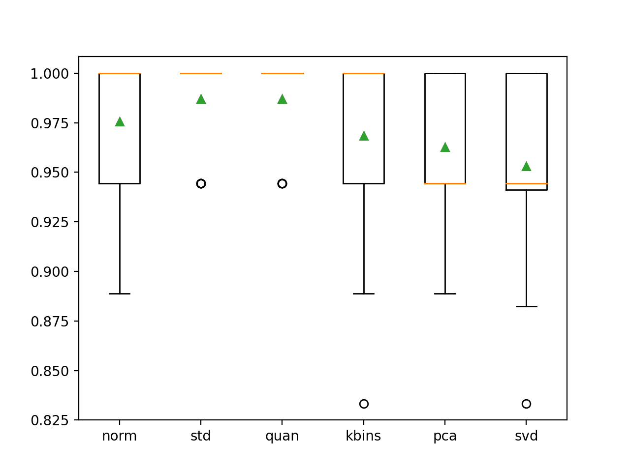
Box and Whisker Plot of Classification Accuracy for Different Data Transforms on the Wine Classification Dataset
We can also explore sequences of transforms to see if they can offer a lift in performance.
For example, we might want to apply RFE feature selection after the standardization transform to see if the same or better results can be used with fewer input variables (e.g. less complexity).
We might also want to see if a power transform preceded with a data scaling transform can achieve good performance on the dataset as we believe it could given the success of the quantile transform.
The updated get_pipelines() function with sequences of transforms is provided below.
# get modeling pipelines to evaluate
def get_pipelines(model):
	pipelines = list()
	# standardize
	p = Pipeline([('s',StandardScaler()), ('r', RFE(estimator=LogisticRegression(solver='liblinear'), n_features_to_select=10)), ('m',model)])
	pipelines.append(('std', p))
	# scale and power
	p = Pipeline([('s',MinMaxScaler((1,2))), ('p', PowerTransformer()), ('m',model)])
	pipelines.append(('power', p))
	return pipelines
Tying this together, the complete example is listed below.
# compare sequences of data preparation methods for the wine classification dataset
from numpy import mean
from numpy import std
from pandas import read_csv
from sklearn.model_selection import RepeatedStratifiedKFold
from sklearn.model_selection import cross_val_score
from sklearn.linear_model import LogisticRegression
from sklearn.pipeline import Pipeline
from sklearn.preprocessing import LabelEncoder
from sklearn.preprocessing import MinMaxScaler
from sklearn.preprocessing import StandardScaler
from sklearn.preprocessing import QuantileTransformer
from sklearn.preprocessing import PowerTransformer
from sklearn.preprocessing import KBinsDiscretizer
from sklearn.decomposition import PCA
from sklearn.decomposition import TruncatedSVD
from sklearn.feature_selection import RFE
from matplotlib import pyplot

# prepare the dataset
def load_dataset():
	# load the dataset
	url = 'https://raw.githubusercontent.com/jbrownlee/Datasets/master/wine.csv'
	df = read_csv(url, header=None)
	data = df.values
	X, y = data[:, :-1], data[:, -1]
	# minimally prepare dataset
	X = X.astype('float')
	y = LabelEncoder().fit_transform(y.astype('str'))
	return X, y

# evaluate a model
def evaluate_model(X, y, model):
	# define the cross-validation procedure
	cv = RepeatedStratifiedKFold(n_splits=10, n_repeats=3, random_state=1)
	# evaluate model
	scores = cross_val_score(model, X, y, scoring='accuracy', cv=cv, n_jobs=-1)
	return scores

# get modeling pipelines to evaluate
def get_pipelines(model):
	pipelines = list()
	# standardize
	p = Pipeline([('s',StandardScaler()), ('r', RFE(estimator=LogisticRegression(solver='liblinear'), n_features_to_select=10)), ('m',model)])
	pipelines.append(('std', p))
	# scale and power
	p = Pipeline([('s',MinMaxScaler((1,2))), ('p', PowerTransformer()), ('m',model)])
	pipelines.append(('power', p))
	return pipelines

# get the dataset
X, y = load_dataset()
# define the model
model = LogisticRegression(solver='liblinear')
# get the modeling pipelines
pipelines = get_pipelines(model)
# evaluate each pipeline
results, names = list(), list()
for name, pipeline in pipelines:
	# evaluate
	scores = evaluate_model(X, y, pipeline)
	# summarize
	print('>%s: %.3f (%.3f)' % (name, mean(scores), std(scores)))
	# store
	results.append(scores)
	names.append(name)
# plot the result
pyplot.boxplot(results, labels=names, showmeans=True)
pyplot.show()
Running the example evaluates the performance of each pipeline and reports the mean and standard deviation classification accuracy.
Your results may vary given the stochastic nature of the learning algorithm, the evaluation procedure, and differences in precision across machines. Try running the example a few times.
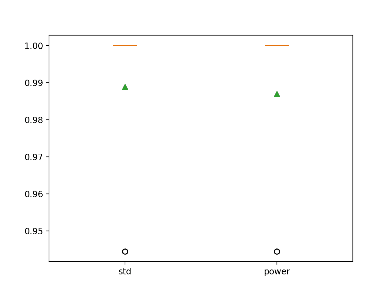
In this case, we can see that the standardization with feature selection offers an additional lift in accuracy from 98.7 percent to 98.9 percent, although the data scaling and power transform do not offer any additional benefit over the quantile transform.
>std: 0.989 (0.022)
>power: 0.987 (0.023)
A figure is created showing box and whisker plots that summarize the distribution of classification accuracy scores for each data preparation technique.
We can see that the distribution of results for both pipelines of transforms is compact with very little spread other than outlier.
Box and Whisker Plot of Classification Accuracy for Different Sequences of Data Transforms on the Wine Classification Dataset
Further Reading
This section provides more resources on the topic if you are looking to go deeper.
Books
APIs
Summary
In this tutorial, you discovered how to use a grid search approach for data preparation with tabular data.
Specifically, you learned:
- Grid search provides an alternative approach to data preparation for tabular data, where transforms are tried as hyperparameters of the modeling pipeline.
- How to use the grid search method for data preparation to improve model performance over a baseline for a standard classification dataset.
- How to grid search sequences of data preparation methods to further improve model performance.
Do you have any questions?
Ask your questions in the comments below and I will do my best to answer.
The post How to Grid Search Data Preparation Techniques appeared first on Machine Learning Mastery.