Author: Adrian Tam
Compared to other programming exercises, a machine learning project is a blend of code and data. You need both to achieve the result and do something useful. Over the years, many well-known datasets have been created, and many have become standards or benchmarks. In this tutorial, we are going to see how we can obtain those well-known public datasets easily. We will also learn how to make a synthetic dataset if none of the existing datasets fits our needs.
After finishing this tutorial, you will know:
- Where to look for freely available datasets for machine learning projects
- How to download datasets using libraries in Python
- How to generate synthetic datasets using scikit-learn
Let’s get started.

A Guide to Getting Datasets for Machine Learning in Python
Photo by Olha Ruskykh. Some rights reserved.
Tutorial Overview
This tutorial is divided into four parts; they are:
- Dataset repositories
- Retrieving dataset in scikit-learn and Seaborn
- Retrieving dataset in TensorFlow
- Generating dataset in scikit-learn
Dataset Repositories
Machine learning has been developed for decades, and therefore there are some datasets of historical significance. One of the most well-known repositories for these datasets is the UCI Machine Learning Repository. Most of the datasets over there are small in size because the technology at the time was not advanced enough to handle larger size data. Some famous datasets located in this repository are the iris flower dataset (introduced by Ronald Fisher in 1936) and the 20 newsgroups dataset (textual data usually referred to by information retrieval literature).
Newer datasets are usually larger in size. For example, the ImageNet dataset is over 160 GB. These datasets are commonly found in Kaggle, and we can search them by name. If we need to download them, it is recommended to use Kaggle’s command line tool after registering for an account.
OpenML is a newer repository that hosts a lot of datasets. It is convenient because you can search for the dataset by name, but it also has a standardized web API for users to retrieve data. It would be useful if you want to use Weka since it provides files in ARFF format.
But still, many datasets are publicly available but not in these repositories for various reasons. You may also want to check out the “List of datasets for machine-learning research” page List of datasets for machine-learning research” on Wikipedia. That page contains a long list of datasets attributed to different categories, with links to download them.
Retrieving Datasets in scikit-learn and Seaborn
Trivially, you may obtain those datasets by downloading them from the web, either through the browser, via command line, using the wget tool, or using network libraries such as requests in Python. Since some of those datasets have become a standard or benchmark, many machine learning libraries have created functions to help retrieve them. For practical reasons, often, the datasets are not shipped with the libraries but downloaded in real time when you invoke the functions. Therefore, you need to have a steady internet connection to use them.
Scikit-learn is an example where you can download the dataset using its API. The related functions are defined under sklearn.datasets,and you may see the list of functions at:
For example, you can use the function load_iris() to get the iris flower dataset as follows:
import sklearn.datasets

data, target = sklearn.datasets.load_iris(return_X_y=True, as_frame=True)
data["target"] = target
print(data)
The load_iris() function would return numpy arrays (i.e., does not have column headers) instead of pandas DataFrame unless the argument as_frame=True is specified. Also, we pass return_X_y=True to the function, so only the machine learning features and targets are returned, rather than some metadata such as the description of the dataset. The above code prints the following:
sepal length (cm)  sepal width (cm)  petal length (cm)  petal width (cm)  target
0                  5.1               3.5                1.4               0.2       0
1                  4.9               3.0                1.4               0.2       0
2                  4.7               3.2                1.3               0.2       0
3                  4.6               3.1                1.5               0.2       0
4                  5.0               3.6                1.4               0.2       0
..                 ...               ...                ...               ...     ...
145                6.7               3.0                5.2               2.3       2
146                6.3               2.5                5.0               1.9       2
147                6.5               3.0                5.2               2.0       2
148                6.2               3.4                5.4               2.3       2
149                5.9               3.0                5.1               1.8       2

[150 rows x 5 columns]
Separating the features and targets is convenient for training a scikit-learn model, but combining them would be helpful for visualization. For example, we may combine the DataFrame as above and then visualize the correlogram using Seaborn:
import sklearn.datasets
import matplotlib.pyplot as plt
import seaborn as sns

data, target = sklearn.datasets.load_iris(return_X_y=True, as_frame=True)
data["target"] = target

sns.pairplot(data, kind="scatter", diag_kind="kde", hue="target",
             palette="muted", plot_kws={'alpha':0.7})
plt.show()
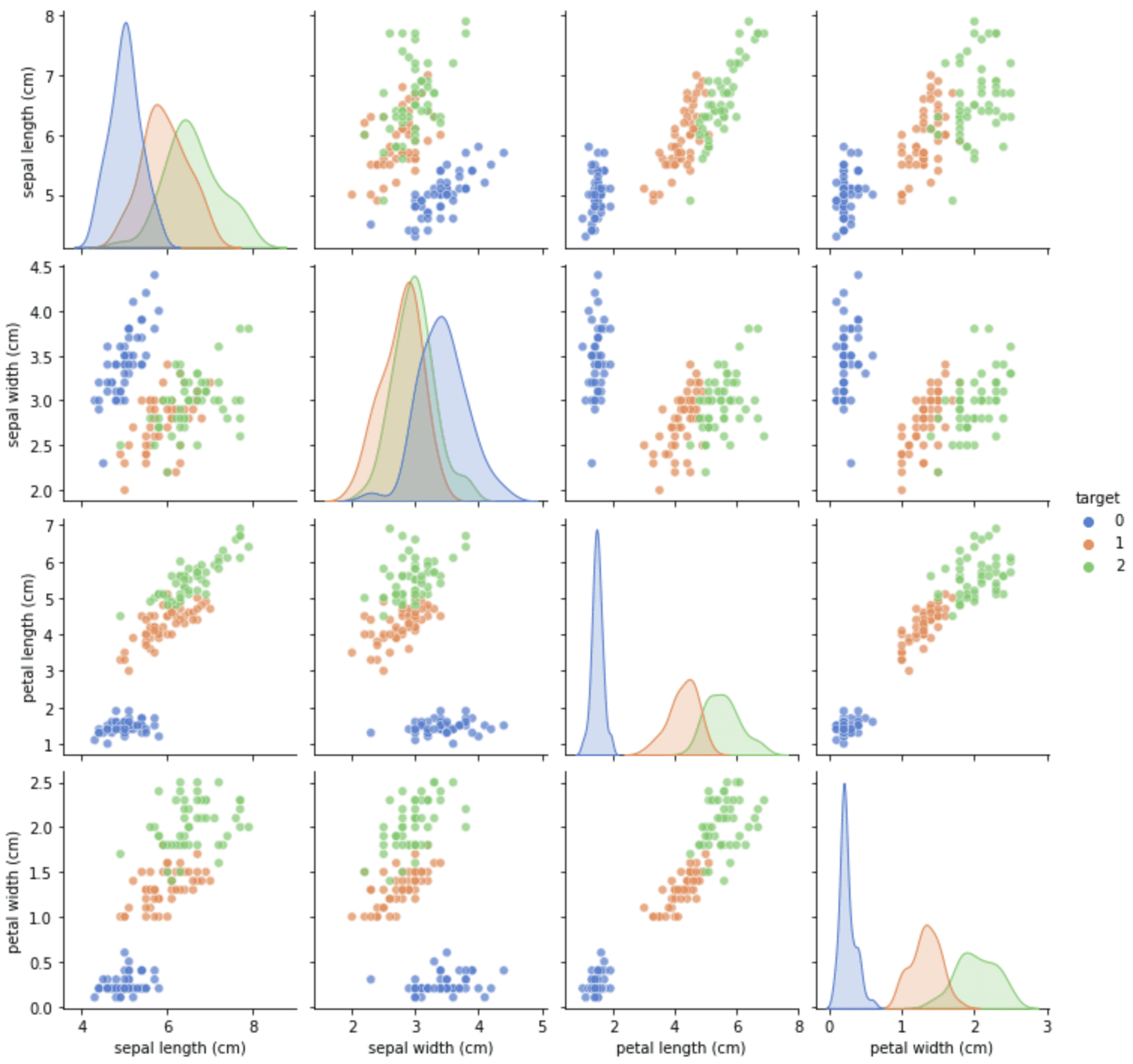
From the correlogram, we can see that target 0 is easy to distinguish, but targets 1 and 2 usually have some overlap. Because this dataset is also useful to demonstrate plotting functions, we can find the equivalent data loading function from Seaborn. We can rewrite the above into the following:
import matplotlib.pyplot as plt
import seaborn as sns

data = sns.load_dataset("iris")
sns.pairplot(data, kind="scatter", diag_kind="kde", hue="species",
             palette="muted", plot_kws={'alpha':0.7})
plt.show()
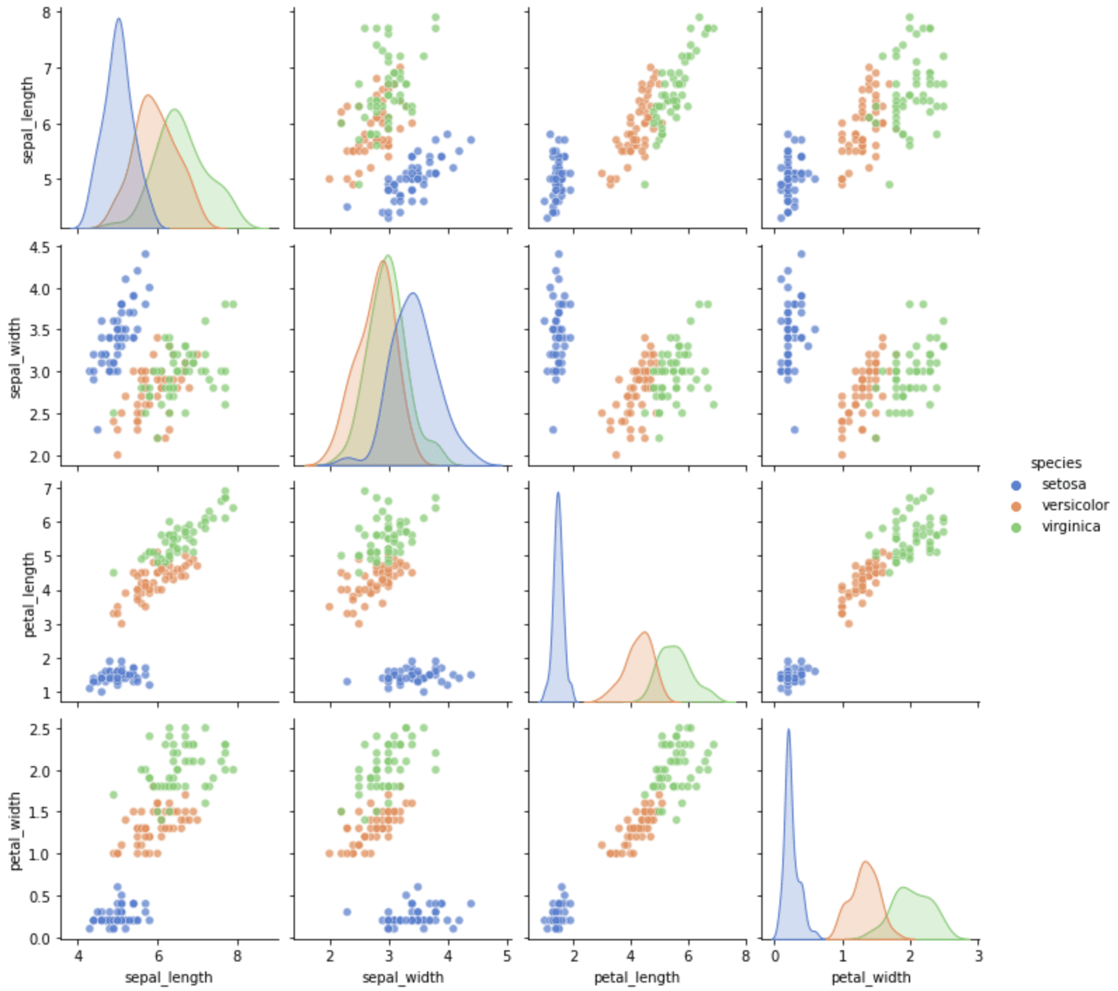
The dataset supported by Seaborn is more limited. We can see the names of all supported datasets by running:
import seaborn as sns
print(sns.get_dataset_names())
where the following is all the datasets from Seaborn:
['anagrams', 'anscombe', 'attention', 'brain_networks', 'car_crashes',
'diamonds', 'dots', 'exercise', 'flights', 'fmri', 'gammas', 'geyser',
'iris', 'mpg', 'penguins', 'planets', 'taxis', 'tips', 'titanic']
There are a handful of similar functions to load the “toy datasets” from scikit-learn. For example, we have load_wine() and load_diabetes() defined in similar fashion.
Larger datasets are also similar. We have fetch_california_housing(), for example, that needs to download the dataset from the internet (hence the “fetch” in the function name). Scikit-learn documentation calls these the “real-world datasets,” but, in fact, the toy datasets are equally real.
import sklearn.datasets

data = sklearn.datasets.fetch_california_housing(return_X_y=False, as_frame=True)
data = data["frame"]
print(data)
MedInc  HouseAge  AveRooms  AveBedrms  Population  AveOccup  Latitude  Longitude  MedHouseVal
0      8.3252      41.0  6.984127   1.023810       322.0  2.555556     37.88    -122.23        4.526
1      8.3014      21.0  6.238137   0.971880      2401.0  2.109842     37.86    -122.22        3.585
2      7.2574      52.0  8.288136   1.073446       496.0  2.802260     37.85    -122.24        3.521
3      5.6431      52.0  5.817352   1.073059       558.0  2.547945     37.85    -122.25        3.413
4      3.8462      52.0  6.281853   1.081081       565.0  2.181467     37.85    -122.25        3.422
...       ...       ...       ...        ...         ...       ...       ...        ...          ...
20635  1.5603      25.0  5.045455   1.133333       845.0  2.560606     39.48    -121.09        0.781
20636  2.5568      18.0  6.114035   1.315789       356.0  3.122807     39.49    -121.21        0.771
20637  1.7000      17.0  5.205543   1.120092      1007.0  2.325635     39.43    -121.22        0.923
20638  1.8672      18.0  5.329513   1.171920       741.0  2.123209     39.43    -121.32        0.847
20639  2.3886      16.0  5.254717   1.162264      1387.0  2.616981     39.37    -121.24        0.894

[20640 rows x 9 columns]
If we need more than these, scikit-learn provides a handy function to read any dataset from OpenML. For example,
import sklearn.datasets

data = sklearn.datasets.fetch_openml("diabetes", version=1, as_frame=True, return_X_y=False)
data = data["frame"]
print(data)
preg   plas  pres  skin   insu  mass   pedi   age            class
0     6.0  148.0  72.0  35.0    0.0  33.6  0.627  50.0  tested_positive
1     1.0   85.0  66.0  29.0    0.0  26.6  0.351  31.0  tested_negative
2     8.0  183.0  64.0   0.0    0.0  23.3  0.672  32.0  tested_positive
3     1.0   89.0  66.0  23.0   94.0  28.1  0.167  21.0  tested_negative
4     0.0  137.0  40.0  35.0  168.0  43.1  2.288  33.0  tested_positive
..    ...    ...   ...   ...    ...   ...    ...   ...              ...
763  10.0  101.0  76.0  48.0  180.0  32.9  0.171  63.0  tested_negative
764   2.0  122.0  70.0  27.0    0.0  36.8  0.340  27.0  tested_negative
765   5.0  121.0  72.0  23.0  112.0  26.2  0.245  30.0  tested_negative
766   1.0  126.0  60.0   0.0    0.0  30.1  0.349  47.0  tested_positive
767   1.0   93.0  70.0  31.0    0.0  30.4  0.315  23.0  tested_negative

[768 rows x 9 columns]
Sometimes, we should not use the name to identify a dataset in OpenML as there may be multiple datasets of the same name. We can search for the data ID on OpenML and use it in the function as follows:
import sklearn.datasets

data = sklearn.datasets.fetch_openml(data_id=42437, return_X_y=False, as_frame=True)
data = data["frame"]
print(data)
The data ID in the code above refers to the titanic dataset. We can extend the code into the following to show how we can obtain the titanic dataset and then run the logistic regression:
from sklearn.linear_model import LogisticRegression
from sklearn.datasets import fetch_openml

X, y = fetch_openml(data_id=42437, return_X_y=True, as_frame=False)
clf = LogisticRegression(random_state=0).fit(X, y)
print(clf.score(X,y)) # accuracy
print(clf.coef_)      # coefficient in logistic regression
0.8114478114478114
[[-0.7551392   2.24013347 -0.20761281  0.28073571  0.24416706 -0.36699113
   0.4782924 ]]
Retrieving Datasets in TensorFlow
Besides scikit-learn, TensorFlow is another tool that we can use for machine learning projects. For similar reasons, there is also a dataset API for TensorFlow that gives you the dataset in a format that works best with TensorFlow. Unlike scikit-learn, the API is not part of the standard TensorFlow package. You need to install it using the command:
pip install tensorflow-datasets
The list of all datasets is available on the catalog:
All datasets are identified by a name. The names can be found in the catalog above. You may also get a list of names using the following:
import tensorflow_datasets as tfds
print(tfds.list_builders())
which prints more than 1,000 names.
As an example, let’s pick the MNIST handwritten digits dataset as an example. We can download the data as follows:
import tensorflow_datasets as tfds
ds = tfds.load("mnist", split="train", shuffle_files=True)
print(ds)
This shows us that tfds.load() gives us an object of type tensorflow.data.OptionsDataset:
<_OptionsDataset shapes: {image: (28, 28, 1), label: ()}, types: {image: tf.uint8, label: tf.int64}>
In particular, this dataset has the data instances (images) in a numpy array of shapes (28,28,1), and the targets (labels) are scalars.
With minor polishing, the data is ready for use in the Keras fit() function. An example is as follows:
import tensorflow as tf
import tensorflow_datasets as tfds
from tensorflow.keras.models import Sequential
from tensorflow.keras.layers import Conv2D, Dense, AveragePooling2D, Dropout, Flatten
from tensorflow.keras.callbacks import EarlyStopping

# Read data with train-test split
ds_train, ds_test = tfds.load("mnist", split=['train', 'test'],
                              shuffle_files=True, as_supervised=True)

# Set up BatchDataset from the OptionsDataset object
ds_train = ds_train.batch(32)
ds_test = ds_test.batch(32)

# Build LeNet5 model and fit
model = Sequential([
    Conv2D(6, (5,5), input_shape=(28,28,1), padding="same", activation="tanh"),
    AveragePooling2D((2,2), strides=2),
    Conv2D(16, (5,5), activation="tanh"),
    AveragePooling2D((2,2), strides=2),
    Conv2D(120, (5,5), activation="tanh"),
    Flatten(),
    Dense(84, activation="tanh"),
    Dense(10, activation="softmax")
])
model.compile(loss="sparse_categorical_crossentropy", optimizer="adam", metrics=["sparse_categorical_accuracy"])
earlystopping = EarlyStopping(monitor="val_loss", patience=2, restore_best_weights=True)
model.fit(ds_train, validation_data=ds_test, epochs=100, callbacks=[earlystopping])
If we provided as_supervised=True, the dataset would be records of tuples (features, targets) instead of the dictionary. It is required for Keras. Moreover, to use the dataset in the fit() function, we need to create an iterable of batches. This is done by setting up the batch size of the dataset to convert it from OptionsDataset object into BatchDataset object.
We applied the LeNet5 model for the image classification. But since the target in the dataset is a numerical value (0 to 9) rather than a Boolean vector, we ask Keras to convert the softmax output vector into a number before computing accuracy and loss by specifying sparse_categorical_accuracy and sparse_categorical_crossentropy in the compile() function.
The key here is to understand every dataset is in a different shape. When you use it with your TensorFlow model, you need to adapt your model to fit the dataset.
Generating Datasets in scikit-learn
In scikit-learn, there is a set of very useful functions to generate a dataset with particular properties. Because we can control the properties of the synthetic dataset, it is helpful to evaluate the performance of our models in a specific situation that is not commonly seen in other datasets.
Scikit-learn documentation calls these functions the samples generator. It is easy to use; for example:
from sklearn.datasets import make_circles
import matplotlib.pyplot as plt

data, target = make_circles(n_samples=500, shuffle=True, factor=0.7, noise=0.1)
plt.figure(figsize=(6,6))
plt.scatter(data[:,0], data[:,1], c=target, alpha=0.8, cmap="Set1")
plt.show()
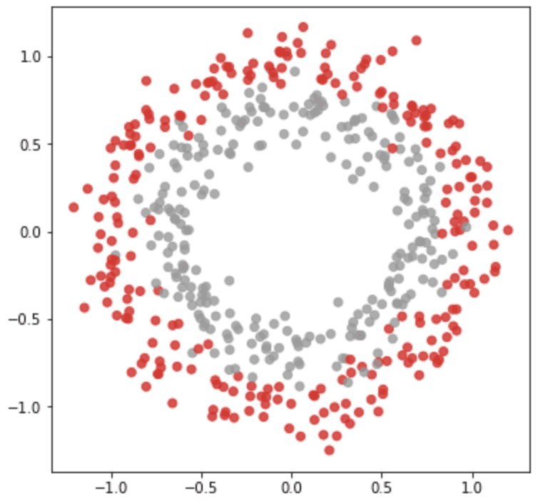
The make_circles() function generates coordinates of scattered points in a 2D plane such that there are two classes positioned in the form of concentric circles. We can control the size and overlap of the circles with the parameters factor and noise in the argument. This synthetic dataset is helpful to evaluate classification models such as a support vector machine since there is no linear separator available.
The output from make_circles() is always in two classes, and the coordinates are always in 2D. But some other functions can generate points of more classes or in higher dimensions, such as make_blob(). In the example below, we generate a dataset in 3D with 4 classes:
from sklearn.datasets import make_blobs
import matplotlib.pyplot as plt

data, target = make_blobs(n_samples=500, n_features=3, centers=4,
                          shuffle=True, random_state=42, cluster_std=2.5)

fig = plt.figure(figsize=(8,8))
ax = fig.add_subplot(projection='3d')
ax.scatter(data[:,0], data[:,1], data[:,2], c=target, alpha=0.7, cmap="Set1")
plt.show()
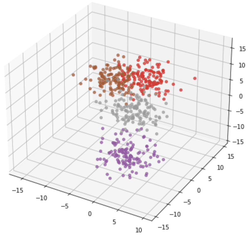
There are also some functions to generate a dataset for regression problems. For example, make_s_curve() and make_swiss_roll() will generate coordinates in 3D with targets as continuous values.
from sklearn.datasets import make_s_curve, make_swiss_roll
import matplotlib.pyplot as plt

data, target = make_s_curve(n_samples=5000, random_state=42)

fig = plt.figure(figsize=(15,8))
ax = fig.add_subplot(121, projection='3d')
ax.scatter(data[:,0], data[:,1], data[:,2], c=target, alpha=0.7, cmap="viridis")

data, target = make_swiss_roll(n_samples=5000, random_state=42)
ax = fig.add_subplot(122, projection='3d')
ax.scatter(data[:,0], data[:,1], data[:,2], c=target, alpha=0.7, cmap="viridis")

plt.show()
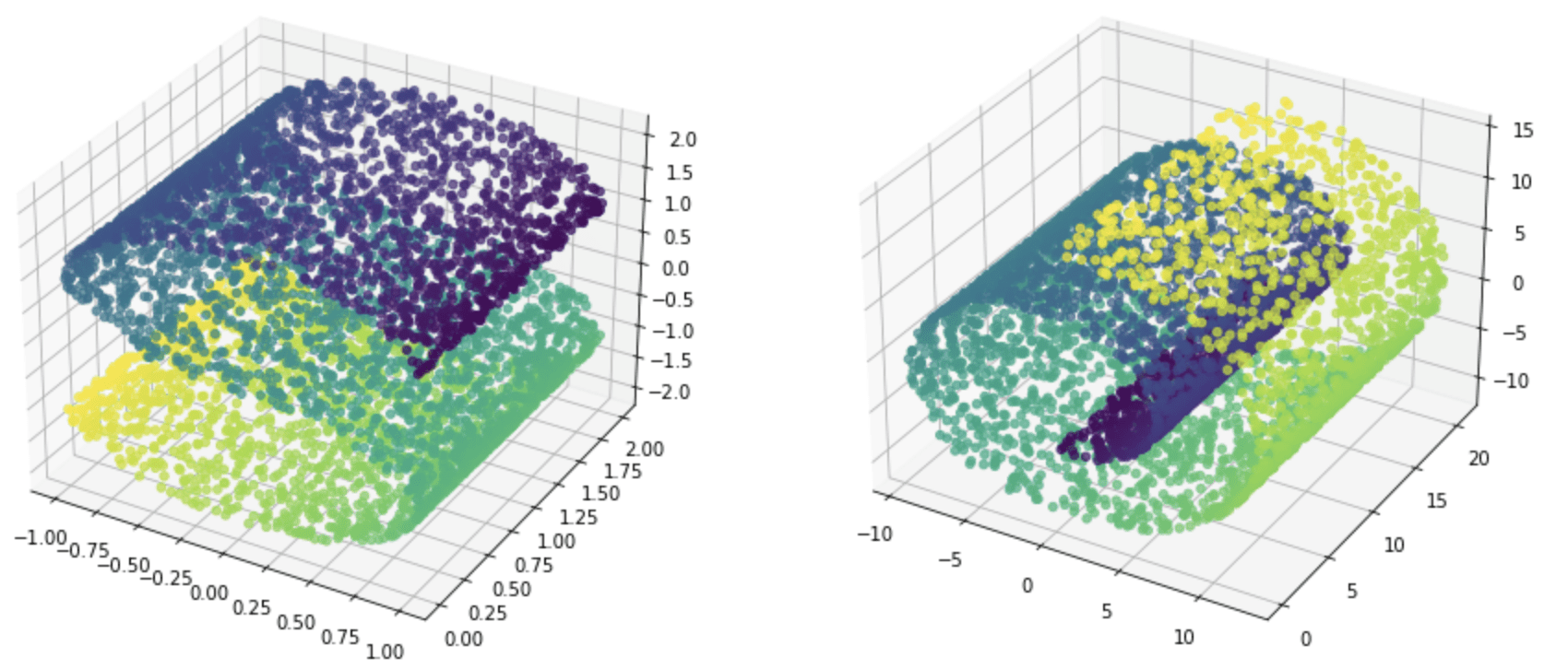
If we prefer not to look at the data from a geometric perspective, there are also make_classification() and make_regression(). Compared to the other functions, these two provide us more control over the feature sets, such as introducing some redundant or irrelevant features.
Below is an example of using make_regression() to generate a dataset and run linear regression with it:
from sklearn.datasets import make_regression
from sklearn.linear_model import LinearRegression
import numpy as np

# Generate 10-dimensional features and 1-dimensional targets
X, y = make_regression(n_samples=500, n_features=10, n_targets=1, n_informative=4,
                       noise=0.5, bias=-2.5, random_state=42)

# Run linear regression on the data
reg = LinearRegression()
reg.fit(X, y)

# Print the coefficient and intercept found
with np.printoptions(precision=5, linewidth=100, suppress=True):
    print(np.array(reg.coef_))
    print(reg.intercept_)
In the example above, we created 10-dimensional features, but only 4 of them are informative. Hence from the result of the regression, we found only 4 of the coefficients are significantly non-zero.
[-0.00435 -0.02232 19.0113   0.04391 46.04906 -0.02882 -0.05692 28.61786 -0.01839 16.79397]
-2.5106367126731413
An example of using make_classification() similarly is as follows. A support vector machine classifier is used in this case:
from sklearn.datasets import make_classification
from sklearn.svm import SVC
import numpy as np

# Generate 10-dimensional features and 3-class targets
X, y = make_classification(n_samples=1000, n_features=10, n_classes=3,
                           n_informative=4, n_redundant=2, n_repeated=1,
                           random_state=42)

# Run SVC on the data
clf = SVC(kernel="rbf")
clf.fit(X, y)

# Print the accuracy
print(clf.score(X, y))
Further Reading
This section provides more resources on the topic if you are looking to go deeper.
Repositories
- UCI machine learning repository
- Kaggle
- OpenML
- Wikipedia, https://en.wikipedia.org/wiki/List_of_datasets_for_machine-learning_research
Articles
- List of datasets for machine-learning research, Wikipedia
- scikit-learn toy datasets
- scikit-learn real-world datasets
- TensorFlow datasets catalog
- Training a neural network on MNIST with Keras using TensorFlow Datasets
APIs
Summary
In this tutorial, you discovered various options for loading a common dataset or generating one in Python.
Specifically, you learned:
- How to use the dataset API in scikit-learn, Seaborn, and TensorFlow to load common machine learning datasets
- The small differences in the format of the dataset returned by different APIs and how to use them
- How to generate a dataset using scikit-learn
The post A Guide to Getting Datasets for Machine Learning in Python appeared first on Machine Learning Mastery.
