
Author: Jason Brownlee
A prediction from a machine learning perspective is a single point that hides the uncertainty of that prediction.
Prediction intervals provide a way to quantify and communicate the uncertainty in a prediction. They are different from confidence intervals that instead seek to quantify the uncertainty in a population parameter such as a mean or standard deviation. Prediction intervals describe the uncertainty for a single specific outcome.
In this tutorial, you will discover the prediction interval and how to calculate it for a simple linear regression model.
After completing this tutorial, you will know:
- That a prediction interval quantifies the uncertainty of a single point prediction.
- That prediction intervals can be estimated analytically for simple models, but are more challenging for nonlinear machine learning models.
- How to calculate the prediction interval for a simple linear regression model.
Let’s get started.

Prediction Intervals for Machine Learning
Photo by Jim Bendon, some rights reserved.
Tutorial Overview
This tutorial is divided into 5 parts; they are:
- What Is Wrong With a Point Estimate?
- What Is a Prediction Interval?
- How to Calculate a Prediction Interval
- Prediction Interval for Linear Regression
- Worked Example
Need help with Statistics for Machine Learning?
Take my free 7-day email crash course now (with sample code).
Click to sign-up and also get a free PDF Ebook version of the course.
Why Calculate a Prediction Interval?
In predictive modeling, a prediction or a forecast is a single outcome value given some input variables.
For example:
yhat = model.predict(X)
Where yhat is the estimated outcome or prediction made by the trained model for the given input data X.
This is a point prediction.
By definition, it is an estimate or an approximation and contains some uncertainty.
The uncertainty comes from the errors in the model itself and noise in the input data. The model is an approximation of the relationship between the input variables and the output variables.
Given the process used to choose and tune the model, it will be the best approximation made given available information, but it will still make errors. Data from the domain will naturally obscure the underlying and unknown relationship between the input and output variables. This will make it a challenge to fit the model, and will also make it a challenge for a fit model to make predictions.
Given these two main sources of error, their point prediction from a predictive model is insufficient for describing the true uncertainty of the prediction.
What Is a Prediction Interval?
A prediction interval is a quantification of the uncertainty on a prediction.
It provides a probabilistic upper and lower bounds on the estimate of an outcome variable.
A prediction interval for a single future observation is an interval that will, with a specified degree of confidence, contain a future randomly selected observation from a distribution.
— Page 27, Statistical Intervals: A Guide for Practitioners and Researchers, 2017.
Prediction intervals are most commonly used when making predictions or forecasts with a regression model, where a quantity is being predicted.
An example of the presentation of a prediction interval is as follows:
Given a prediction of ‘y’ given ‘x’, there is a 95% likelihood that the range ‘a’ to ‘b’ covers the true outcome.
The prediction interval surrounds the prediction made by the model and hopefully covers the range of the true outcome.
The diagram below helps to visually understand the relationship between the prediction, prediction interval, and the actual outcome.
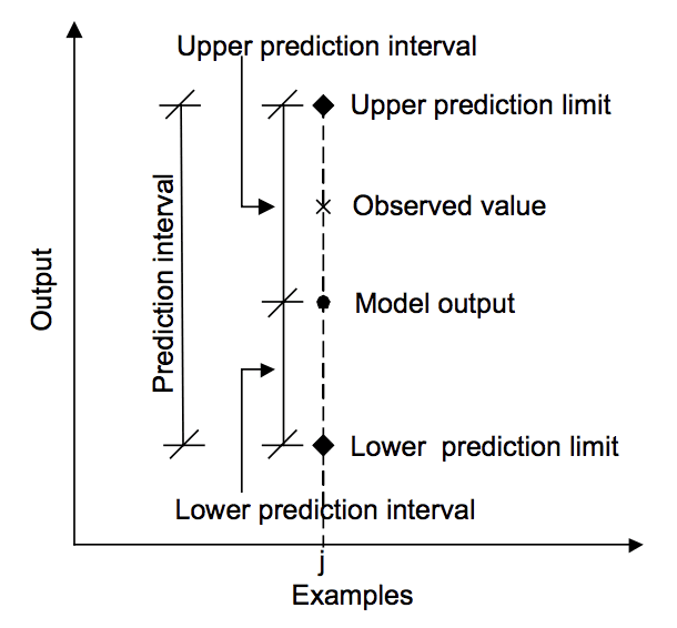
Relationship between prediction, actual value and prediction interval.
Taken from “Machine learning approaches for estimation of prediction interval for the model output”, 2006.
A prediction interval is different from a confidence interval.
A confidence interval quantifies the uncertainty on an estimated population variable, such as the mean or standard deviation. Whereas a prediction interval quantifies the uncertainty on a single observation estimated from the population.
In predictive modeling, a confidence interval can be used to quantify the uncertainty of the estimated skill of a model, whereas a prediction interval can be used to quantify the uncertainty of a single forecast.
A prediction interval is often larger than the confidence interval as it must take the confidence interval and the variance in the output variable being predicted into account.
Prediction intervals will always be wider than confidence intervals because they account for the uncertainty associated with e [error], the irreducible error.
— Page 103, An Introduction to Statistical Learning: with Applications in R, 2013.
How to Calculate a Prediction Interval
A prediction interval is calculated as some combination of the estimated variance of the model and the variance of the outcome variable.
Prediction intervals are easy to describe, but difficult to calculate in practice.
In simple cases like linear regression, we can estimate the confidence interval directly.
In the cases of nonlinear regression algorithms, such as artificial neural networks, it is a lot more challenging and requires the choice and implementation of specialized techniques. General techniques such as the bootstrap resampling method can be used, but are computationally expensive to calculate.
The paper “A Comprehensive Review of Neural Network-based Prediction Intervals and New Advances” provides a reasonably recent study of prediction intervals for nonlinear models in the context of neural networks. The following list summarizes some methods that can be used for prediction uncertainty for nonlinear machine learning models:
- The Delta Method, from the field of nonlinear regression.
- The Bayesian Method, from Bayesian modeling and statistics.
- The Mean-Variance Estimation Method, using estimated statistics.
- The Bootstrap Method, using data resampling and developing an ensemble of models.
We can make the calculation of a prediction interval concrete with a worked example in the next section.
Prediction Interval for Linear Regression
A linear regression is a model that describes the linear combination of inputs to calculate the output variables.
For example, an estimated linear regression model may be written as:
yhat = b0 + b1 . x
Where yhat is the prediction, b0 and b1 are coefficients of the model estimated from training data and x is the input variable.
We do not know the true values of the coefficients b0 and b1. We also do not know the true population parameters such as mean and standard deviation for x or y. All of these elements must be estimated, which introduces uncertainty into the use of the model in order to make predictions.
We can make some assumptions, such as the distributions of x and y and the prediction errors made by the model, called residuals, are Gaussian.
The prediction interval around yhat can be calculated as follows:
yhat +/- z * sigma
Where yhat is the predicted value, z is the critical value from the Gaussian distribution (e.g. 1.96 for a 95% interval) and sigma is the standard deviation of the predicted distribution.
We do not known in practice. We can calculate an unbiased estimate of the of the predicted standard deviation as follows (taken from Machine learning approaches for estimation of prediction interval for the model output):
stdev = sqrt(1 / (N - 2) * e(i)^2 for i to N)
Where stdev is an unbiased estimate of the standard deviation for the predicted distribution, n are the total predictions made, and e(i) is the difference between the ith prediction and actual value.
Worked Example
Let’s make the case of linear regression prediction intervals concrete with a worked example.
First, let’s define a simple two-variable dataset where the output variable (y) depends on the input variable (x) with some Gaussian noise.
The example below defines the dataset we will use for this example.
# generate related variables
from numpy import mean
from numpy import std
from numpy.random import randn
from numpy.random import seed
from matplotlib import pyplot
# seed random number generator
seed(1)
# prepare data
x = 20 * randn(1000) + 100
y = x + (10 * randn(1000) + 50)
# summarize
print('x: mean=%.3f stdv=%.3f' % (mean(x), std(x)))
print('y: mean=%.3f stdv=%.3f' % (mean(y), std(y)))
# plot
pyplot.scatter(x, y)
pyplot.show()
Running the example first prints the mean and standard deviations of the two variables.
x: mean=100.776 stdv=19.620
y: mean=151.050 stdv=22.358
A plot of the dataset is then created.
We can see the clear linear relationship between the variables with the spread of the points highlighting the noise or random error in the relationship.

Scatter Plot of Related Variables
Next, we can develop a simple linear regression that given the input variable x, will predict the y variable. We can use the linregress() SciPy function to fit the model and return the b0 and b1 coefficients for the model.
# fit linear regression model
b1, b0, r_value, p_value, std_err = linregress(x, y)
We can use the coefficients to calculate the predicted y values, called yhat, for each of the input variables. The resulting points will form a line that represents the learned relationship.
# make prediction
yhat = b0 + b1 * x
The complete example is listed below.
# simple linear regression model
from numpy.random import randn
from numpy.random import seed
from scipy.stats import linregress
from matplotlib import pyplot
# seed random number generator
seed(1)
# prepare data
x = 20 * randn(1000) + 100
y = x + (10 * randn(1000) + 50)
# fit linear regression model
b1, b0, r_value, p_value, std_err = linregress(x, y)
print('b0=%.3f, b1=%.3f' % (b1, b0))
# make prediction
yhat = b0 + b1 * x
# plot data and predictions
pyplot.scatter(x, y)
pyplot.plot(x, yhat, color='r')
pyplot.show()
Running the example fits the model and prints the coefficients.
b0=1.011, b1=49.117
The coefficients are then used with the inputs from the dataset to make a prediction. The resulting inputs and predicted y-values are plotted as a line on top of the scatter plot for the dataset.
We can clearly see that the model has learned the underlying relationship in the dataset.
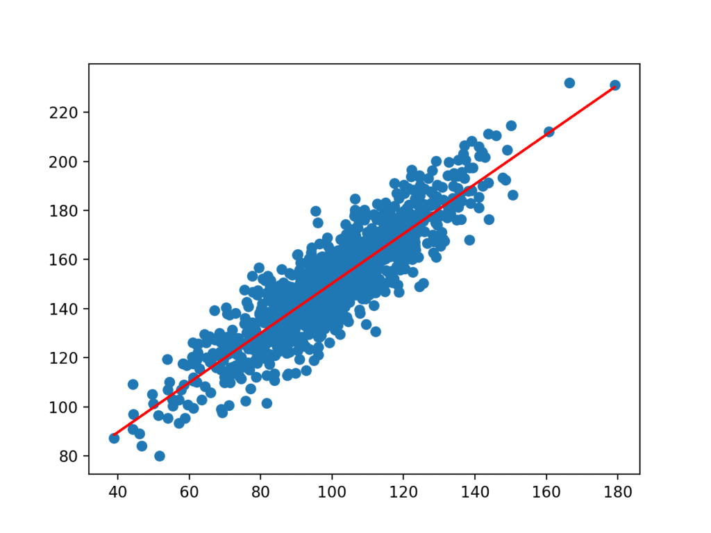
Scatter Plot of Dataset with Line for Simple Linear Regression Model
We are now ready to make a prediction with our simple linear regression model and add a prediction interval.
We will fit the model as before. This time we will take one sample from the dataset to demonstrate the prediction interval. We will use the input to make a prediction, calculate the prediction interval for the prediction, and compare the prediction and interval to the known expected value.
First, let’s define the input, prediction, and expected values.
x_in = x[0]
y_out = y[0]
yhat_out = yhat[0]
Next, we can estimate the standard deviation in the prediction direction.
SE = sqrt(1 / (N - 2) * e(i)^2 for i to N)
We can calculate this directly using the NumPy arrays as follows:
# estimate stdev of yhat
sum_errs = arraysum((y - yhat)**2)
stdev = sqrt(1/(len(y)-2) * sum_errs)
Next, we can calculate the prediction interval for our chosen input:
interval = z . stdev
We will use the significance level of 95%, which is the Gaussian critical value of 1.69.
Once the interval is calculated, we can summarize the bounds on the prediction to the user.
# calculate prediction interval
interval = 1.96 * stdev
lower, upper = y_out - interval, y_out + interval
We can tie all of this together. The complete example is listed below.
# linear regression prediction with prediction interval
from numpy.random import randn
from numpy.random import seed
from numpy import power
from numpy import sqrt
from numpy import mean
from numpy import std
from numpy import sum as arraysum
from scipy.stats import linregress
from matplotlib import pyplot
# seed random number generator
seed(1)
# prepare data
x = 20 * randn(1000) + 100
y = x + (10 * randn(1000) + 50)
# fit linear regression model
b1, b0, r_value, p_value, std_err = linregress(x, y)
# make predictions
yhat = b0 + b1 * x
# define new input, expected value and prediction
x_in = x[0]
y_out = y[0]
yhat_out = yhat[0]
# estimate stdev of yhat
sum_errs = arraysum((y - yhat)**2)
stdev = sqrt(1/(len(y)-2) * sum_errs)
# calculate prediction interval
interval = 1.96 * stdev
print('Prediction Interval: %.3f' % interval)
lower, upper = y_out - interval, y_out + interval
print('95%% likelihood that the true value is between %.3f and %.3f' % (lower, upper))
print('True value: %.3f' % yhat_out)
# plot dataset and prediction with interval
pyplot.scatter(x, y)
pyplot.plot(x, yhat, color='red')
pyplot.errorbar(x_in, yhat_out, yerr=interval, color='black', fmt='o')
pyplot.show()
Running the example estimates the yhat standard deviation and then calculates the confidence interval.
Once calculated, the prediction interval is presented to the user for the given input variable. Because we contrived this example, we know the true outcome, which we also display. We can see that in this case, the 95% prediction interval does cover the true expected value.
linear regression model.},style=None]
Prediction Interval: 20.204
95% likelihood that the true value is between 160.750 and 201.159
True value: 183.124
A plot is also created showing the raw dataset as a scatter plot, the predictions for the dataset as a red line, and the prediction and prediction interval as a black dot and line respectively.
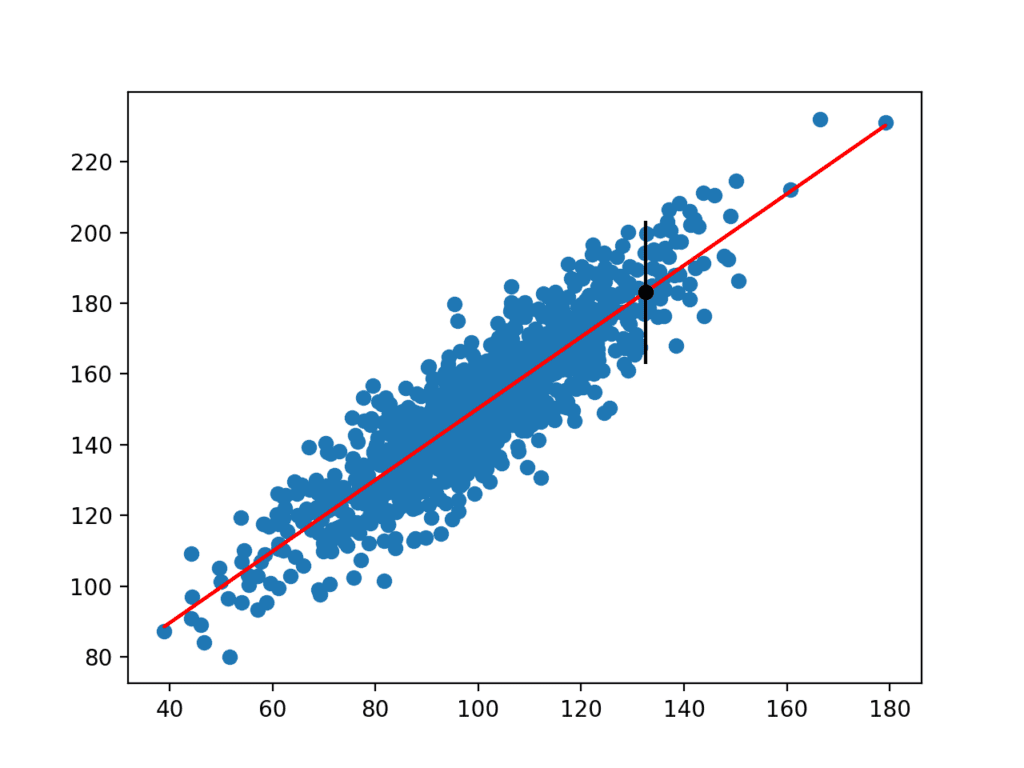
Scatter Plot of Dataset With Linear Model and Prediction Interval
Extensions
This section lists some ideas for extending the tutorial that you may wish to explore.
- Summarize the difference between tolerance, confidence, and prediction intervals.
- Develop a linear regression model for a standard machine learning dataset and calculate prediction intervals for a small test set.
- Describe in detail how one nonlinear prediction interval method works.
If you explore any of these extensions, I’d love to know.
Further Reading
This section provides more resources on the topic if you are looking to go deeper.
Posts
- How to Report Classifier Performance with Confidence Intervals
- How to Calculate Bootstrap Confidence Intervals For Machine Learning Results in Python
- Understand Time Series Forecast Uncertainty Using Confidence Intervals with Python
- Estimate the Number of Experiment Repeats for Stochastic Machine Learning Algorithms
Books
- Understanding The New Statistics: Effect Sizes, Confidence Intervals, and Meta-Analysis, 2017.
- Statistical Intervals: A Guide for Practitioners and Researchers, 2017.
- An Introduction to Statistical Learning: with Applications in R, 2013.
- Introduction to the New Statistics: Estimation, Open Science, and Beyond, 2016.
- Forecasting: principles and practice, 2013.
Papers
- A comparison of some error estimates for neural network models, 1995.
- Machine learning approaches for estimation of prediction interval for the model output, 2006.
- A Comprehensive Review of Neural Network-based Prediction Intervals and New Advances, 2010.
API
Articles
Summary
In this tutorial, you discovered the prediction interval and how to calculate it for a simple linear regression model.
Specifically, you learned:
- That a prediction interval quantifies the uncertainty of a single point prediction.
- That prediction intervals can be estimated analytically for simple models but are more challenging for nonlinear machine learning models.
- How to calculate the prediction interval for a simple linear regression model.
Do you have any questions?
Ask your questions in the comments below and I will do my best to answer.
The post Prediction Intervals for Machine Learning appeared first on Machine Learning Mastery.