Author: Jason Brownlee
Machine learning algorithms like Linear Regression and Gaussian Naive Bayes assume the numerical variables have a Gaussian probability distribution.
Your data may not have a Gaussian distribution and instead may have a Gaussian-like distribution (e.g. nearly Gaussian but with outliers or a skew) or a totally different distribution (e.g. exponential).
As such, you may be able to achieve better performance on a wide range of machine learning algorithms by transforming input and/or output variables to have a Gaussian or more-Gaussian distribution. Power transforms like the Box-Cox transform and the Yeo-Johnson transform provide an automatic way of performing these transforms on your data and are provided in the scikit-learn Python machine learning library.
In this tutorial, you will discover how to use power transforms in scikit-learn to make variables more Gaussian for modeling.
After completing this tutorial, you will know:
- Many machine learning algorithms prefer or perform better when numerical variables have a Gaussian probability distribution.
- Power transforms are a technique for transforming numerical input or output variables to have a Gaussian or more-Gaussian-like probability distribution.
- How to use the PowerTransform in scikit-learn to use the Box-Cox and Yeo-Johnson transforms when preparing data for predictive modeling.
Let’s get started.

How to Use Power Transforms With scikit-learn
Photo by Ian D. Keating, some rights reserved.
Tutorial Overview
This tutorial is divided into five parts; they are:
- Make Data More Gaussian
- Power Transforms
- Sonar Dataset
- Box-Cox Transform
- Yeo-Johnson Transform
Make Data More Gaussian
Many machine learning algorithms perform better when the distribution of variables is Gaussian.
Recall that the observations for each variable may be thought to be drawn from a probability distribution. The Gaussian is a common distribution with the familiar bell shape. It is so common that it is often referred to as the “normal” distribution.
For more on the Gaussian probability distribution, see the tutorial:
Some algorithms like linear regression and logistic regression explicitly assume the real-valued variables have a Gaussian distribution. Other nonlinear algorithms may not have this assumption, yet often perform better when variables have a Gaussian distribution.
This applies both to real-valued input variables in the case of classification and regression tasks, and real-valued target variables in the case of regression tasks.
There are data preparation techniques that can be used to transform each variable to make the distribution Gaussian, or if not Gaussian, then more Gaussian like.
These transforms are most effective when the data distribution is nearly-Gaussian to begin with and is afflicted with a skew or outliers.
Another common reason for transformations is to remove distributional skewness. An un-skewed distribution is one that is roughly symmetric. This means that the probability of falling on either side of the distribution’s mean is roughly equal
— Page 31, Applied Predictive Modeling, 2013.
Power transforms refer to a class of techniques that use a power function (like a logarithm or exponent) to make the probability distribution of a variable Gaussian or more-Gaussian like.
For more on the topic of making variables Gaussian, see the tutorial:
Power Transforms
A power transform will make the probability distribution of a variable more Gaussian.
This is often described as removing a skew in the distribution, although more generally is described as stabilizing the variance of the distribution.
The log transform is a specific example of a family of transformations known as power transforms. In statistical terms, these are variance-stabilizing transformations.
— Page 23, Feature Engineering for Machine Learning, 2018.
We can apply a power transform directly by calculating the log or square root of the variable, although this may or may not be the best power transform for a given variable.
Replacing the data with the log, square root, or inverse may help to remove the skew.
— Page 31, Applied Predictive Modeling, 2013.
Instead, we can use a generalized version of the transform that finds a parameter (lambda) that best transforms a variable to a Gaussian probability distribution.
There are two popular approaches for such automatic power transforms; they are:
- Box-Cox Transform
- Yeo-Johnson Transform
The transformed training dataset can then be fed to a machine learning model to learn a predictive modeling task.
A hyperparameter, often referred to as lambda is used to control the nature of the transform.
… statistical methods can be used to empirically identify an appropriate transformation. Box and Cox (1964) propose a family of transformations that are indexed by a parameter, denoted as lambda
— Page 32, Applied Predictive Modeling, 2013.
Below are some common values for lambda
- lambda = -1. is a reciprocal transform.
- lambda = -0.5 is a reciprocal square root transform.
- lambda = 0.0 is a log transform.
- lambda = 0.5 is a square root transform.
- lambda = 1.0 is no transform.
The optimal value for this hyperparameter used in the transform for each variable can be stored and reused to transform new data in the future in an identical manner, such as a test dataset or new data in the future.
These power transforms are available in the scikit-learn Python machine learning library via the PowerTransformer class.
The class takes an argument named “method” that can be set to ‘yeo-johnson‘ or ‘box-cox‘ for the preferred method. It will also standardize the data automatically after the transform, meaning each variable will have a zero mean and unit variance. This can be turned off by setting the “standardize” argument to False.
We can demonstrate the PowerTransformer with a small worked example. We can generate a sample of random Gaussian numbers and impose a skew on the distribution by calculating the exponent. The PowerTransformer can then be used to automatically remove the skew from the data.
The complete example is listed below.
# demonstration of the power transform on data with a skew
from numpy import exp
from numpy.random import randn
from sklearn.preprocessing import PowerTransformer
from matplotlib import pyplot
# generate gaussian data sample
data = randn(1000)
# add a skew to the data distribution
data = exp(data)
# histogram of the raw data with a skew
pyplot.hist(data, bins=25)
pyplot.show()
# reshape data to have rows and columns
data = data.reshape((len(data),1))
# power transform the raw data
power = PowerTransformer(method='yeo-johnson', standardize=True)
data_trans = power.fit_transform(data)
# histogram of the transformed data
pyplot.hist(data_trans, bins=25)
pyplot.show()
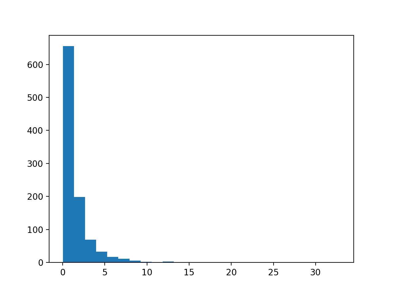
Running the example first creates a sample of 1,000 random Gaussian values and adds a skew to the dataset.
A histogram is created from the skewed dataset and clearly shows the distribution pushed to the far left.

Histogram of Skewed Gaussian Distribution
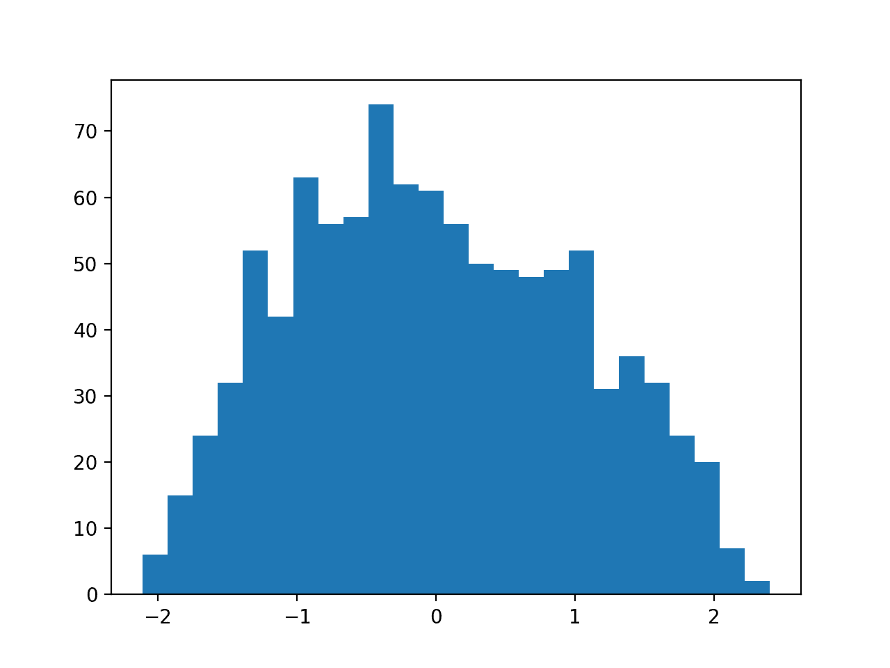
Then a PowerTransformer is used to make the data distribution more-Gaussian and standardize the result, centering the values on the mean value of 0 and a standard deviation of 1.0.
A histogram of the transform data is created showing a more-Gaussian shaped data distribution.

Histogram of Skewed Gaussian Data After Power Transform
In the following sections will take a closer look at how to use these two power transforms on a real dataset.
Next, let’s introduce the dataset.
Sonar Dataset
The sonar dataset is a standard machine learning dataset for binary classification.
It involves 60 real-valued inputs and a 2-class target variable. There are 208 examples in the dataset and the classes are reasonably balanced.
A baseline classification algorithm can achieve a classification accuracy of about 53.4 percent using repeated stratified 10-fold cross-validation. Top performance on this dataset is about 88 percent using repeated stratified 10-fold cross-validation.
The dataset describes radar returns of rocks or simulated mines.
You can learn more about the dataset from here:
No need to download the dataset; we will download it automatically from our worked examples.
First, let’s load and summarize the dataset. The complete example is listed below.
# load and summarize the sonar dataset
from pandas import read_csv
from pandas.plotting import scatter_matrix
from matplotlib import pyplot
# Load dataset
url = "https://raw.githubusercontent.com/jbrownlee/Datasets/master/sonar.csv"
dataset = read_csv(url, header=None)
# summarize the shape of the dataset
print(dataset.shape)
# summarize each variable
print(dataset.describe())
# histograms of the variables
dataset.hist()
pyplot.show()
Running the example first summarizes the shape of the loaded dataset.
This confirms the 60 input variables, one output variable, and 208 rows of data.
A statistical summary of the input variables is provided showing that values are numeric and range approximately from 0 to 1.
(208, 61)
               0           1           2   ...          57          58          59
count  208.000000  208.000000  208.000000  ...  208.000000  208.000000  208.000000
mean     0.029164    0.038437    0.043832  ...    0.007949    0.007941    0.006507
std      0.022991    0.032960    0.038428  ...    0.006470    0.006181    0.005031
min      0.001500    0.000600    0.001500  ...    0.000300    0.000100    0.000600
25%      0.013350    0.016450    0.018950  ...    0.003600    0.003675    0.003100
50%      0.022800    0.030800    0.034300  ...    0.005800    0.006400    0.005300
75%      0.035550    0.047950    0.057950  ...    0.010350    0.010325    0.008525
max      0.137100    0.233900    0.305900  ...    0.044000    0.036400    0.043900

[8 rows x 60 columns]
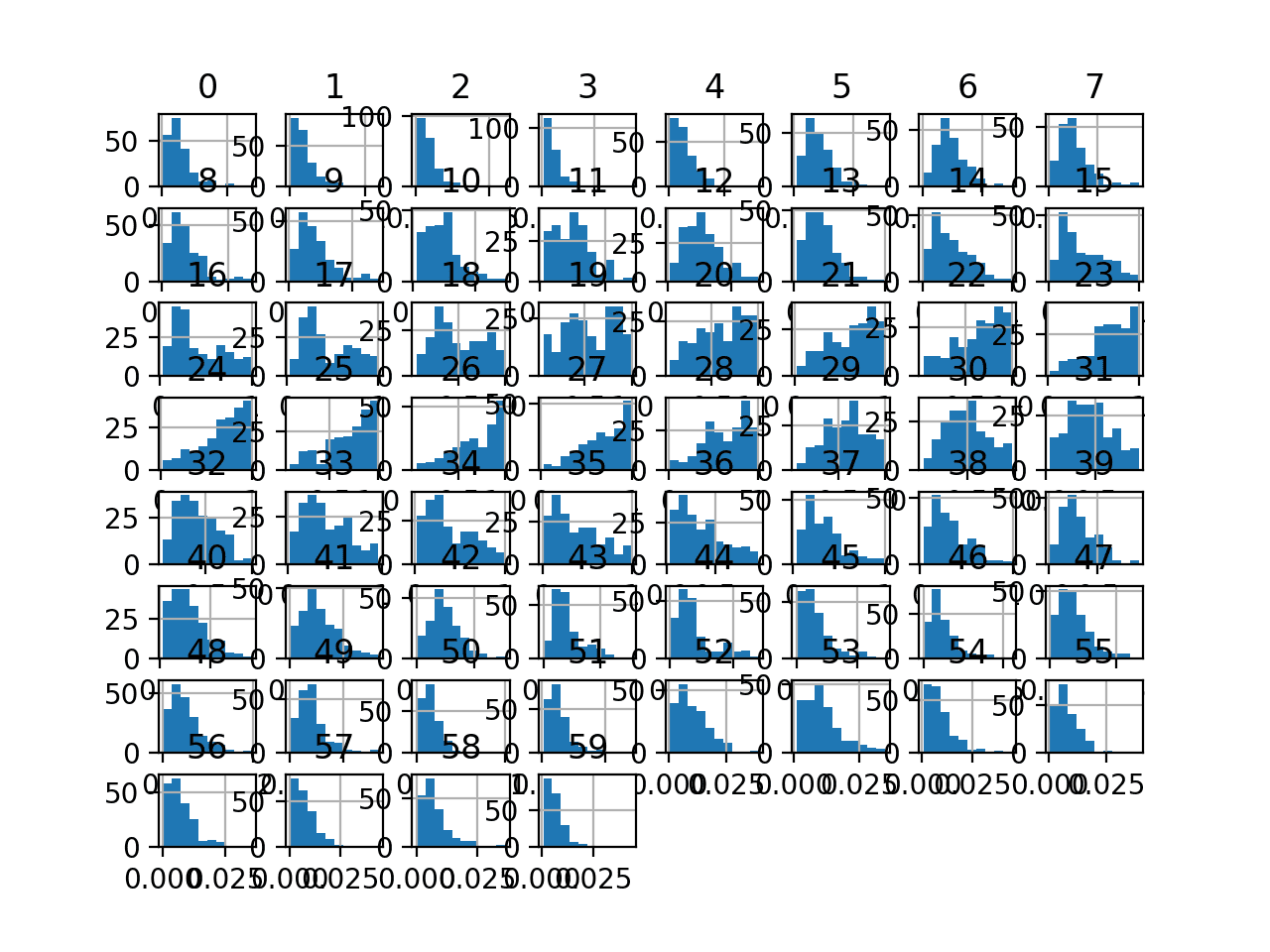
Finally, a histogram is created for each input variable.
If we ignore the clutter of the plots and focus on the histograms themselves, we can see that many variables have a skewed distribution.
The dataset provides a good candidate for using a power transform to make the variables more-Gaussian.

Histogram Plots of Input Variables for the Sonar Binary Classification Dataset
Next, let’s fit and evaluate a machine learning model on the raw dataset.
We will use a k-nearest neighbor algorithm with default hyperparameters and evaluate it using repeated stratified k-fold cross-validation. The complete example is listed below.
# evaluate knn on the raw sonar dataset
from numpy import mean
from numpy import std
from pandas import read_csv
from sklearn.model_selection import cross_val_score
from sklearn.model_selection import RepeatedStratifiedKFold
from sklearn.neighbors import KNeighborsClassifier
from sklearn.preprocessing import LabelEncoder
from matplotlib import pyplot
# load dataset
url = "https://raw.githubusercontent.com/jbrownlee/Datasets/master/sonar.csv"
dataset = read_csv(url, header=None)
data = dataset.values
# separate into input and output columns
X, y = data[:, :-1], data[:, -1]
# ensure inputs are floats and output is an integer label
X = X.astype('float32')
y = LabelEncoder().fit_transform(y.astype('str'))
# define and configure the model
model = KNeighborsClassifier()
# evaluate the model
cv = RepeatedStratifiedKFold(n_splits=10, n_repeats=3, random_state=1)
n_scores = cross_val_score(model, X, y, scoring='accuracy', cv=cv, n_jobs=-1, error_score='raise')
# report model performance
print('Accuracy: %.3f (%.3f)' % (mean(n_scores), std(n_scores)))
Running the example evaluates a KNN model on the raw sonar dataset.
We can see that the model achieved a mean classification accuracy of about 79.7 percent, showing that it has skill (better than 53.4 percent) and is in the ball-park of good performance (88 percent).
Accuracy: 0.797 (0.073)
Next, let’s explore a Box-Cox power transform of the dataset.
Box-Cox Transform
The Box-Cox transform is named for the two authors of the method.
It is a power transform that assumes the values of the input variable to which it is applied are strictly positive. That means 0 and negative values are not supported.
It is important to note that the Box-Cox procedure can only be applied to data that is strictly positive.
— Page 123, Feature Engineering and Selection, 2019.
We can apply the Box-Cox transform using the PowerTransformer class and setting the “method” argument to “box-cox“. Once defined, we can call the fit_transform() function and pass it to our dataset to create a Box-Cox transformed version of our dataset.
...
pt = PowerTransformer(method='box-cox')
data = pt.fit_transform(data)
Our dataset does not have negative values but may have zero values. This may cause a problem.
Let’s try anyway.
The complete example of creating a Box-Cox transform of the sonar dataset and plotting histograms of the result is listed below.
# visualize a box-cox transform of the sonar dataset
from pandas import read_csv
from pandas import DataFrame
from pandas.plotting import scatter_matrix
from sklearn.preprocessing import PowerTransformer
from matplotlib import pyplot
# Load dataset
url = "https://raw.githubusercontent.com/jbrownlee/Datasets/master/sonar.csv"
dataset = read_csv(url, header=None)
# retrieve just the numeric input values
data = dataset.values[:, :-1]
# perform a box-cox transform of the dataset
pt = PowerTransformer(method='box-cox')
data = pt.fit_transform(data)
# convert the array back to a dataframe
dataset = DataFrame(data)
# histograms of the variables
dataset.hist()
pyplot.show()
Running the example results in an error as follows:
ValueError: The Box-Cox transformation can only be applied to strictly positive data
As expected, we cannot use the transform on the raw data because it is not strictly positive.
One way to solve this problem is to use a MixMaxScaler transform first to scale the data to positive values, then apply the transform.
We can use a Pipeline object to apply both transforms in sequence; for example:
...
# perform a box-cox transform of the dataset
scaler = MinMaxScaler(feature_range=(1, 2))
power = PowerTransformer(method='box-cox')
pipeline = Pipeline(steps=[('s', scaler),('p', power)])
data = pipeline.fit_transform(data)
The updated version of applying the Box-Cox transform to the scaled dataset is listed below.
# visualize a box-cox transform of the scaled sonar dataset
from pandas import read_csv
from pandas import DataFrame
from pandas.plotting import scatter_matrix
from sklearn.preprocessing import PowerTransformer
from sklearn.preprocessing import MinMaxScaler
from sklearn.pipeline import Pipeline
from matplotlib import pyplot
# Load dataset
url = "https://raw.githubusercontent.com/jbrownlee/Datasets/master/sonar.csv"
dataset = read_csv(url, header=None)
# retrieve just the numeric input values
data = dataset.values[:, :-1]
# perform a box-cox transform of the dataset
scaler = MinMaxScaler(feature_range=(1, 2))
power = PowerTransformer(method='box-cox')
pipeline = Pipeline(steps=[('s', scaler),('p', power)])
data = pipeline.fit_transform(data)
# convert the array back to a dataframe
dataset = DataFrame(data)
# histograms of the variables
dataset.hist()
pyplot.show()
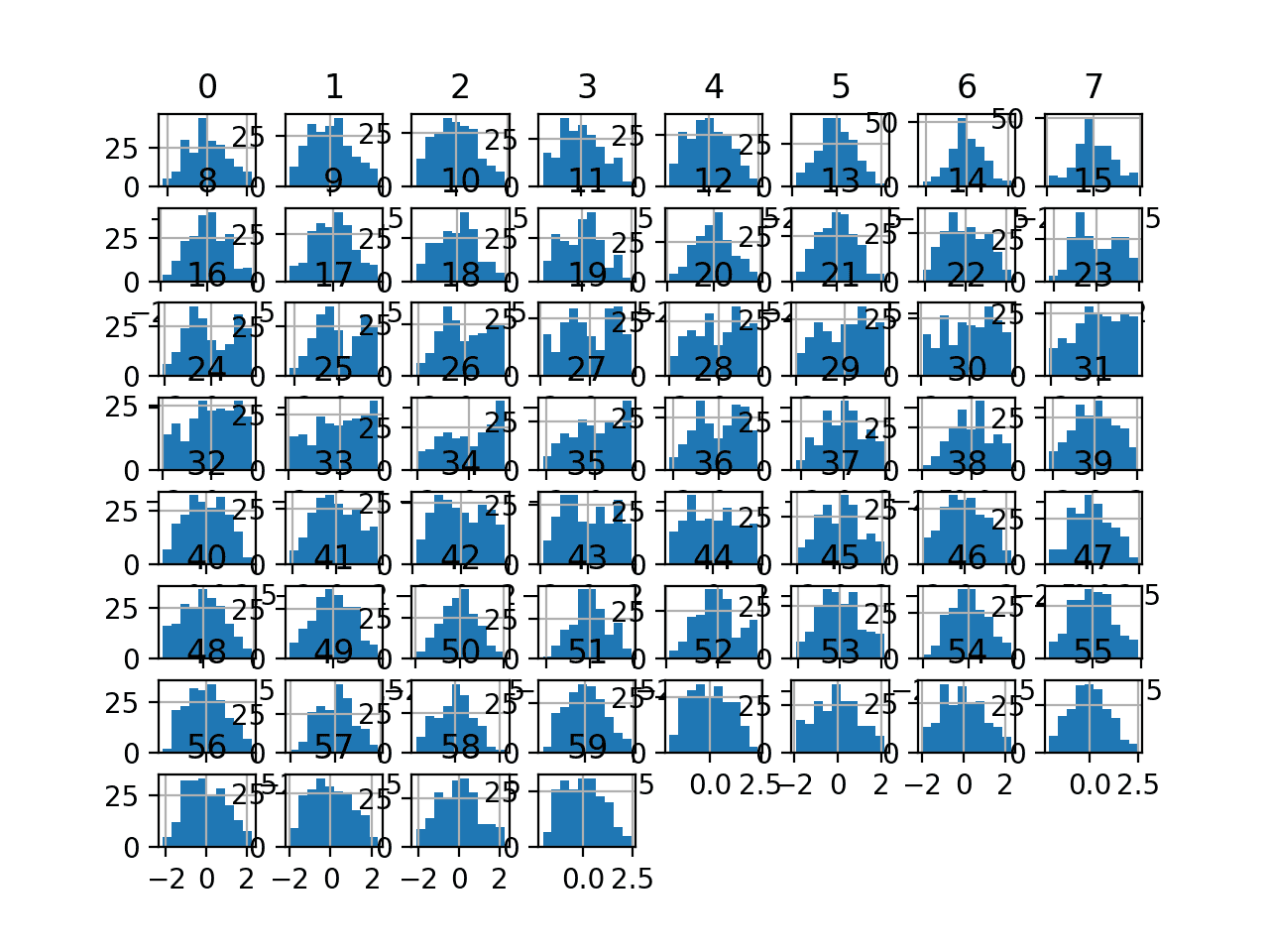
Running the example transforms the dataset and plots histograms of each input variable.
We can see that the shape of the histograms for each variable looks more Gaussian than the raw data.

Histogram Plots of Box-Cox Transformed Input Variables for the Sonar Dataset
Next, let’s evaluate the same KNN model as the previous section, but in this case on a Box-Cox transform of the scaled dataset.
The complete example is listed below.
# evaluate knn on the box-cox sonar dataset
from numpy import mean
from numpy import std
from pandas import read_csv
from sklearn.model_selection import cross_val_score
from sklearn.model_selection import RepeatedStratifiedKFold
from sklearn.neighbors import KNeighborsClassifier
from sklearn.preprocessing import LabelEncoder
from sklearn.preprocessing import PowerTransformer
from sklearn.preprocessing import MinMaxScaler
from sklearn.pipeline import Pipeline
from matplotlib import pyplot
# load dataset
url = "https://raw.githubusercontent.com/jbrownlee/Datasets/master/sonar.csv"
dataset = read_csv(url, header=None)
data = dataset.values
# separate into input and output columns
X, y = data[:, :-1], data[:, -1]
# ensure inputs are floats and output is an integer label
X = X.astype('float32')
y = LabelEncoder().fit_transform(y.astype('str'))
# define the pipeline
scaler = MinMaxScaler(feature_range=(1, 2))
power = PowerTransformer(method='box-cox')
model = KNeighborsClassifier()
pipeline = Pipeline(steps=[('s', scaler),('p', power), ('m', model)])
# evaluate the pipeline
cv = RepeatedStratifiedKFold(n_splits=10, n_repeats=3, random_state=1)
n_scores = cross_val_score(pipeline, X, y, scoring='accuracy', cv=cv, n_jobs=-1, error_score='raise')
# report pipeline performance
print('Accuracy: %.3f (%.3f)' % (mean(n_scores), std(n_scores)))
Running the example, we can see that the Box-Cox transform results in a lift in performance from 79.7 percent accuracy without the transform to about 81.1 percent with the transform.
Accuracy: 0.811 (0.085)
Next, let’s take a closer look at the Yeo-Johnson transform.
Yeo-Johnson Transform
The Yeo-Johnson transform is also named for the authors.
Unlike the Box-Cox transform, it does not require the values for each input variable to be strictly positive. It supports zero values and negative values. This means we can apply it to our dataset without scaling it first.
We can apply the transform by defining a PowerTransform object and setting the “method” argument to “yeo-johnson” (the default).
...
# perform a yeo-johnson transform of the dataset
pt = PowerTransformer(method='yeo-johnson')
data = pt.fit_transform(data)
The example below applies the Yeo-Johnson transform and creates histogram plots of each of the transformed variables.
# visualize a yeo-johnson transform of the sonar dataset
from pandas import read_csv
from pandas import DataFrame
from pandas.plotting import scatter_matrix
from sklearn.preprocessing import PowerTransformer
from matplotlib import pyplot
# Load dataset
url = "https://raw.githubusercontent.com/jbrownlee/Datasets/master/sonar.csv"
dataset = read_csv(url, header=None)
# retrieve just the numeric input values
data = dataset.values[:, :-1]
# perform a yeo-johnson transform of the dataset
pt = PowerTransformer(method='yeo-johnson')
data = pt.fit_transform(data)
# convert the array back to a dataframe
dataset = DataFrame(data)
# histograms of the variables
dataset.hist()
pyplot.show()
Running the example transforms the dataset and plots histograms of each input variable.
We can see that the shape of the histograms for each variable look more Gaussian than the raw data, much like the box-cox transform.

Histogram Plots of Yeo-Johnson Transformed Input Variables for the Sonar Dataset
Next, let’s evaluate the same KNN model as the previous section, but in this case on a Yeo-Johnson transform of the raw dataset.
The complete example is listed below.
# evaluate knn on the yeo-johnson sonar dataset
from numpy import mean
from numpy import std
from pandas import read_csv
from sklearn.model_selection import cross_val_score
from sklearn.model_selection import RepeatedStratifiedKFold
from sklearn.neighbors import KNeighborsClassifier
from sklearn.preprocessing import LabelEncoder
from sklearn.preprocessing import PowerTransformer
from sklearn.preprocessing import MinMaxScaler
from sklearn.pipeline import Pipeline
from matplotlib import pyplot
# load dataset
url = "https://raw.githubusercontent.com/jbrownlee/Datasets/master/sonar.csv"
dataset = read_csv(url, header=None)
data = dataset.values
# separate into input and output columns
X, y = data[:, :-1], data[:, -1]
# ensure inputs are floats and output is an integer label
X = X.astype('float32')
y = LabelEncoder().fit_transform(y.astype('str'))
# define the pipeline
power = PowerTransformer(method='yeo-johnson')
model = KNeighborsClassifier()
pipeline = Pipeline(steps=[('p', power), ('m', model)])
# evaluate the pipeline
cv = RepeatedStratifiedKFold(n_splits=10, n_repeats=3, random_state=1)
n_scores = cross_val_score(pipeline, X, y, scoring='accuracy', cv=cv, n_jobs=-1, error_score='raise')
# report pipeline performance
print('Accuracy: %.3f (%.3f)' % (mean(n_scores), std(n_scores)))
Running the example, we can see that the Yeo-Johnson transform results in a lift in performance from 79.7 percent accuracy without the transform to about 80.8 percent with the transform, less than the Box-Cox transform that achieved about 81.1 percent.
Accuracy: 0.808 (0.082)
Sometimes a lift in performance can be achieved by first standardizing the raw dataset prior to performing a Yeo-Johnson transform.
We can explore this by adding a StandardScaler as a first step in the pipeline.
The complete example is listed below.
# evaluate knn on the yeo-johnson standardized sonar dataset
from numpy import mean
from numpy import std
from pandas import read_csv
from sklearn.model_selection import cross_val_score
from sklearn.model_selection import RepeatedStratifiedKFold
from sklearn.neighbors import KNeighborsClassifier
from sklearn.preprocessing import LabelEncoder
from sklearn.preprocessing import PowerTransformer
from sklearn.preprocessing import StandardScaler
from sklearn.pipeline import Pipeline
from matplotlib import pyplot
# load dataset
url = "https://raw.githubusercontent.com/jbrownlee/Datasets/master/sonar.csv"
dataset = read_csv(url, header=None)
data = dataset.values
# separate into input and output columns
X, y = data[:, :-1], data[:, -1]
# ensure inputs are floats and output is an integer label
X = X.astype('float32')
y = LabelEncoder().fit_transform(y.astype('str'))
# define the pipeline
scaler = StandardScaler()
power = PowerTransformer(method='yeo-johnson')
model = KNeighborsClassifier()
pipeline = Pipeline(steps=[('s', scaler), ('p', power), ('m', model)])
# evaluate the pipeline
cv = RepeatedStratifiedKFold(n_splits=10, n_repeats=3, random_state=1)
n_scores = cross_val_score(pipeline, X, y, scoring='accuracy', cv=cv, n_jobs=-1, error_score='raise')
# report pipeline performance
print('Accuracy: %.3f (%.3f)' % (mean(n_scores), std(n_scores)))
Running the example, we can see that standardizing the data prior to the Yeo-Johnson transform resulted in a small lift in performance from about 80.8 percent to about 81.6 percent, a small lift over the results for the Box-Cox transform.
Accuracy: 0.816 (0.077)
Further Reading
This section provides more resources on the topic if you are looking to go deeper.
Tutorials
- Continuous Probability Distributions for Machine Learning
- How to Use Power Transforms for Time Series Forecast Data with Python
- How to Transform Target Variables for Regression With Scikit-Learn
- How to Transform Data to Better Fit The Normal Distribution
- 4 Common Machine Learning Data Transforms for Time Series Forecasting
Books
- Feature Engineering for Machine Learning, 2018.
- Applied Predictive Modeling, 2013.
- Feature Engineering and Selection, 2019.
Dataset
APIs
Articles
Summary
In this tutorial, you discovered how to use power transforms in scikit-learn to make variables more Gaussian for modeling.
Specifically, you learned:
- Many machine learning algorithms prefer or perform better when numerical variables have a Gaussian probability distribution.
- Power transforms are a technique for transforming numerical input or output variables to have a Gaussian or more-Gaussian-like probability distribution.
- How to use the PowerTransform in scikit-learn to use the Box-Cox and Yeo-Johnson transforms when preparing data for predictive modeling.
Do you have any questions?
Ask your questions in the comments below and I will do my best to answer.
The post How to Use Power Transforms for Machine Learning appeared first on Machine Learning Mastery.
