Multi-Class Imbalanced Classification

Imbalanced classification are those prediction tasks where the distribution of examples across class labels is not equal.

Most imbalanced classification examples focus on binary classification tasks, yet many of the tools and techniques for imbalanced classification also directly support multi-class classification problems.

In this tutorial, you will discover how to use the tools of imbalanced classification with a multi-class dataset.

After completing this tutorial, you will know:

• About the glass identification standard imbalanced multi-class prediction problem.
• How to use SMOTE oversampling for imbalanced multi-class classification.
• How to use cost-sensitive learning for imbalanced multi-class classification.

Discover SMOTE, one-class classification, cost-sensitive learning, threshold moving, and much more in my new book, with 30 step-by-step tutorials and full Python source code.

Let’s get started.

Tutorial Overview

This tutorial is divided into three parts; they are:

1. Glass Multi-Class Classification Dataset
2. SMOTE Oversampling for Multi-Class Classification
3. Cost-Sensitive Learning for Multi-Class Classification

Glass Multi-Class Classification Dataset

In this tutorial, we will focus on the standard imbalanced multi-class classification problem referred to as “Glass Identification” or simply “glass.”

The dataset describes the chemical properties of glass and involves classifying samples of glass using their chemical properties as one of six classes. The dataset was credited to Vina Spiehler in 1987.

Ignoring the sample identification number, there are nine input variables that summarize the properties of the glass dataset; they are:

• RI: Refractive Index
• Na: Sodium
• Mg: Magnesium
• Al: Aluminum
• Si: Silicon
• K: Potassium
• Ca: Calcium
• Ba: Barium
• Fe: Iron

The chemical compositions are measured as the weight percent in corresponding oxide.

There are seven types of glass listed; they are:

• Class 1: building windows (float processed)
• Class 2: building windows (non-float processed)
• Class 3: vehicle windows (float processed)
• Class 4: vehicle windows (non-float processed)
• Class 5: containers
• Class 6: tableware
• Class 7: headlamps

Float glass refers to the process used to make the glass.

There are 214 observations in the dataset and the number of observations in each class is imbalanced. Note that there are no examples for class 4 (non-float processed vehicle windows) in the dataset.

• Class 1: 70 examples
• Class 2: 76 examples
• Class 3: 17 examples
• Class 4: 0 examples
• Class 5: 13 examples
• Class 6: 9 examples
• Class 7: 29 examples

Although there are minority classes, all classes are equally important in this prediction problem.

The dataset can be divided into window glass (classes 1-4) and non-window glass (classes 5-7). There are 163 examples of window glass and 51 examples of non-window glass.

• Window Glass: 163 examples
• Non-Window Glass: 51 examples

Another division of the observations would be between float processed glass and non-float processed glass, in the case of window glass only. This division is more balanced.

• Float Glass: 87 examples
• Non-Float Glass: 76 examples

You can learn more about the dataset here:

• Glass Dataset (glass.csv)
• Glass Dataset Description (glass.names)

No need to download the dataset; we will download it automatically as part of the worked examples.

Below is a sample of the first few rows of the data.

1.52101,13.64,4.49,1.10,71.78,0.06,8.75,0.00,0.00,1
1.51761,13.89,3.60,1.36,72.73,0.48,7.83,0.00,0.00,1
1.51618,13.53,3.55,1.54,72.99,0.39,7.78,0.00,0.00,1
1.51766,13.21,3.69,1.29,72.61,0.57,8.22,0.00,0.00,1
1.51742,13.27,3.62,1.24,73.08,0.55,8.07,0.00,0.00,1
...

We can see that all inputs are numeric and the target variable in the final column is the integer encoded class label.

You can learn more about how to work through this dataset as part of a project in the tutorial:

• Imbalanced Multiclass Classification with the Glass Identification Dataset

Now that we are familiar with the glass multi-class classification dataset, let’s explore how we can use standard imbalanced classification tools with it.

Want to Get Started With Imbalance Classification?

Take my free 7-day email crash course now (with sample code).

Click to sign-up and also get a free PDF Ebook version of the course.

Download Your FREE Mini-Course

SMOTE Oversampling for Multi-Class Classification

Oversampling refers to copying or synthesizing new examples of the minority classes so that the number of examples in the minority class better resembles or matches the number of examples in the majority classes.

Perhaps the most widely used approach to synthesizing new examples is called the Synthetic Minority Oversampling TEchnique, or SMOTE for short. This technique was described by Nitesh Chawla, et al. in their 2002 paper named for the technique titled “SMOTE: Synthetic Minority Over-sampling Technique.”

You can learn more about SMOTE in the tutorial:

• SMOTE for Imbalanced Classification with Python

The imbalanced-learn library provides an implementation of SMOTE that we can use that is compatible with the popular scikit-learn library.

First, the library must be installed. We can install it using pip as follows:

sudo pip install imbalanced-learn

We can confirm that the installation was successful by printing the version of the installed library:

# check version number
import imblearn
print(imblearn.__version__)

Running the example will print the version number of the installed library; for example:

0.6.2

Before we apply SMOTE, let’s first load the dataset and confirm the number of examples in each class.

# load and summarize the dataset
from pandas import read_csv
from collections import Counter
from matplotlib import pyplot
from sklearn.preprocessing import LabelEncoder
# define the dataset location
url = 'https://raw.githubusercontent.com/jbrownlee/Datasets/master/glass.csv'
# load the csv file as a data frame
df = read_csv(url, header=None)
data = df.values
# split into input and output elements
X, y = data[:, :-1], data[:, -1]
# label encode the target variable
y = LabelEncoder().fit_transform(y)
# summarize distribution
counter = Counter(y)
for k,v in counter.items():
	per = v / len(y) * 100
	print('Class=%d, n=%d (%.3f%%)' % (k, v, per))
# plot the distribution
pyplot.bar(counter.keys(), counter.values())
pyplot.show()

Running the example first downloads the dataset and splits it into train and test sets.

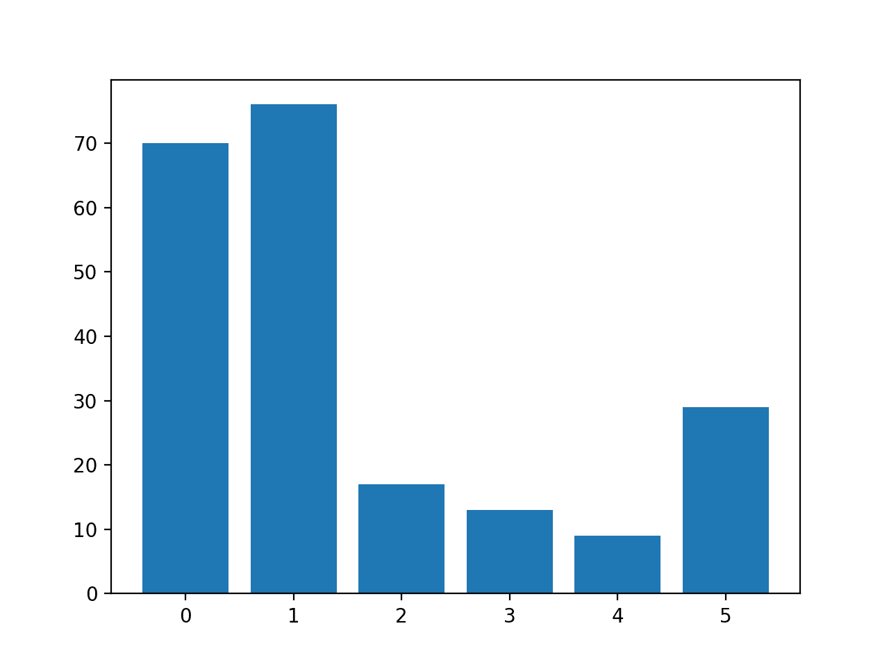
The number of rows in each class is then reported, confirming that some classes, such as 0 and 1, have many more examples (more than 70) than other classes, such as 3 and 4 (less than 15).

Class=0, n=70 (32.710%)
Class=1, n=76 (35.514%)
Class=2, n=17 (7.944%)
Class=3, n=13 (6.075%)
Class=4, n=9 (4.206%)
Class=5, n=29 (13.551%)

A bar chart is created providing a visualization of the class breakdown of the dataset.

This gives a clearer idea that classes 0 and 1 have many more examples than classes 2, 3, 4 and 5.

Next, we can apply SMOTE to oversample the dataset.

By default, SMOTE will oversample all classes to have the same number of examples as the class with the most examples.

In this case, class 1 has the most examples with 76, therefore, SMOTE will oversample all classes to have 76 examples.

The complete example of oversampling the glass dataset with SMOTE is listed below.

# example of oversampling a multi-class classification dataset
from pandas import read_csv
from imblearn.over_sampling import SMOTE
from collections import Counter
from matplotlib import pyplot
from sklearn.preprocessing import LabelEncoder
# define the dataset location
url = 'https://raw.githubusercontent.com/jbrownlee/Datasets/master/glass.csv'
# load the csv file as a data frame
df = read_csv(url, header=None)
data = df.values
# split into input and output elements
X, y = data[:, :-1], data[:, -1]
# label encode the target variable
y = LabelEncoder().fit_transform(y)
# transform the dataset
oversample = SMOTE()
X, y = oversample.fit_resample(X, y)
# summarize distribution
counter = Counter(y)
for k,v in counter.items():
	per = v / len(y) * 100
	print('Class=%d, n=%d (%.3f%%)' % (k, v, per))
# plot the distribution
pyplot.bar(counter.keys(), counter.values())
pyplot.show()

Running the example first loads the dataset and applies SMOTE to it.

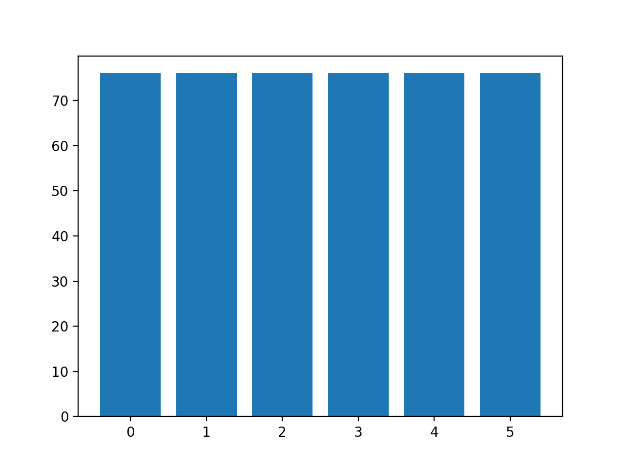
The distribution of examples in each class is then reported, confirming that each class now has 76 examples, as we expected.

Class=0, n=76 (16.667%)
Class=1, n=76 (16.667%)
Class=2, n=76 (16.667%)
Class=3, n=76 (16.667%)
Class=4, n=76 (16.667%)
Class=5, n=76 (16.667%)

A bar chart of the class distribution is also created, providing a strong visual indication that all classes now have the same number of examples.

Instead of using the default strategy of SMOTE to oversample all classes to the number of examples in the majority class, we could instead specify the number of examples to oversample in each class.

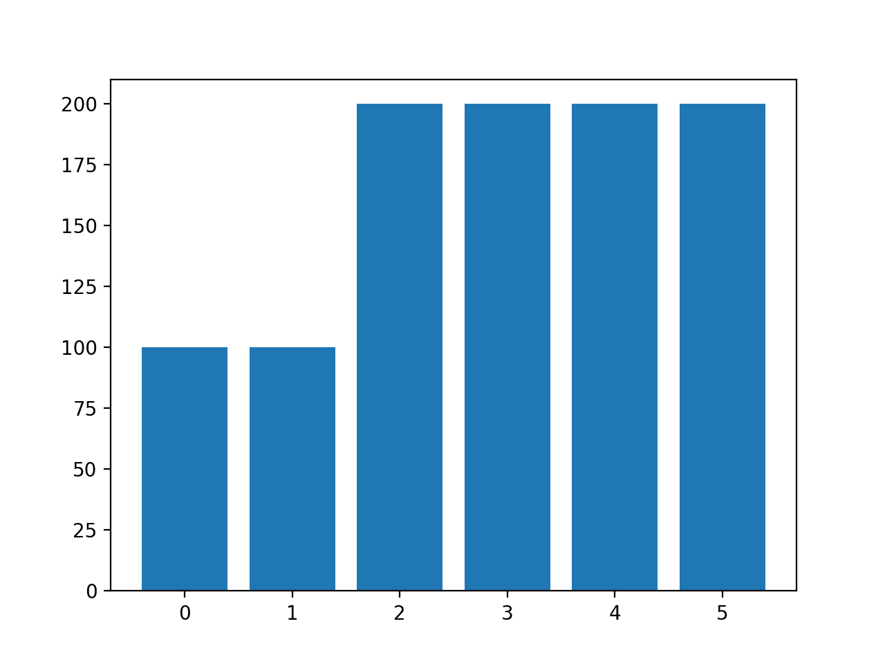
For example, we could oversample to 100 examples in classes 0 and 1 and 200 examples in remaining classes. This can be achieved by creating a dictionary that maps class labels to the number of desired examples in each class, then specifying this via the “sampling_strategy” argument to the SMOTE class.

...
# transform the dataset
strategy = {0:100, 1:100, 2:200, 3:200, 4:200, 5:200}
oversample = SMOTE(sampling_strategy=strategy)
X, y = oversample.fit_resample(X, y)

Tying this together, the complete example of using a custom oversampling strategy for SMOTE is listed below.

# example of oversampling a multi-class classification dataset with a custom strategy
from pandas import read_csv
from imblearn.over_sampling import SMOTE
from collections import Counter
from matplotlib import pyplot
from sklearn.preprocessing import LabelEncoder
# define the dataset location
url = 'https://raw.githubusercontent.com/jbrownlee/Datasets/master/glass.csv'
# load the csv file as a data frame
df = read_csv(url, header=None)
data = df.values
# split into input and output elements
X, y = data[:, :-1], data[:, -1]
# label encode the target variable
y = LabelEncoder().fit_transform(y)
# transform the dataset
strategy = {0:100, 1:100, 2:200, 3:200, 4:200, 5:200}
oversample = SMOTE(sampling_strategy=strategy)
X, y = oversample.fit_resample(X, y)
# summarize distribution
counter = Counter(y)
for k,v in counter.items():
	per = v / len(y) * 100
	print('Class=%d, n=%d (%.3f%%)' % (k, v, per))
# plot the distribution
pyplot.bar(counter.keys(), counter.values())
pyplot.show()

Running the example creates the desired sampling and summarizes the effect on the dataset, confirming the intended result.

Class=0, n=100 (10.000%)
Class=1, n=100 (10.000%)
Class=2, n=200 (20.000%)
Class=3, n=200 (20.000%)
Class=4, n=200 (20.000%)
Class=5, n=200 (20.000%)

Note: you may see warnings that can be safely ignored for the purposes of this example, such as:

UserWarning: After over-sampling, the number of samples (200) in class 5 will be larger than the number of samples in the majority class (class #1 -> 76)

A bar chart of the class distribution is also created confirming the specified class distribution after data sampling.

Note: when using data sampling like SMOTE, it must only be applied to the training dataset, not the entire dataset. I recommend using a Pipeline to ensure that the SMOTE method is correctly used when evaluating models and making predictions with models.

You can see an example of the correct usage of SMOTE in a Pipeline in this tutorial:

• SMOTE for Imbalanced Classification with Python

Cost-Sensitive Learning for Multi-Class Classification

Most machine learning algorithms assume that all classes have an equal number of examples.

This is not the case in multi-class imbalanced classification. Algorithms can be modified to change the way learning is performed to bias towards those classes that have fewer examples in the training dataset. This is generally called cost-sensitive learning.

For more on cost-sensitive learning, see the tutorial:

• Cost-Sensitive Learning for Imbalanced Classification

The RandomForestClassifier class in scikit-learn supports cost-sensitive learning via the “class_weight” argument.

By default, the random forest class assigns equal weight to each class.

We can evaluate the classification accuracy of the default random forest class weighting on the glass imbalanced multi-class classification dataset.

The complete example is listed below.

# baseline model and test harness for the glass identification dataset
from numpy import mean
from numpy import std
from pandas import read_csv
from sklearn.preprocessing import LabelEncoder
from sklearn.model_selection import cross_val_score
from sklearn.model_selection import RepeatedStratifiedKFold
from sklearn.ensemble import RandomForestClassifier

# load the dataset
def load_dataset(full_path):
	# load the dataset as a numpy array
	data = read_csv(full_path, header=None)
	# retrieve numpy array
	data = data.values
	# split into input and output elements
	X, y = data[:, :-1], data[:, -1]
	# label encode the target variable to have the classes 0 and 1
	y = LabelEncoder().fit_transform(y)
	return X, y

# evaluate a model
def evaluate_model(X, y, model):
	# define evaluation procedure
	cv = RepeatedStratifiedKFold(n_splits=5, n_repeats=3, random_state=1)
	# evaluate model
	scores = cross_val_score(model, X, y, scoring='accuracy', cv=cv, n_jobs=-1)
	return scores

# define the location of the dataset
full_path = 'https://raw.githubusercontent.com/jbrownlee/Datasets/master/glass.csv'
# load the dataset
X, y = load_dataset(full_path)
# define the reference model
model = RandomForestClassifier(n_estimators=1000)
# evaluate the model
scores = evaluate_model(X, y, model)
# summarize performance
print('Mean Accuracy: %.3f (%.3f)' % (mean(scores), std(scores)))

Running the example evaluates the default random forest algorithm with 1,000 trees on the glass dataset using repeated stratified k-fold cross-validation.

The mean and standard deviation classification accuracy are reported at the end of the run.

Your specific results may vary given the stochastic nature of the learning algorithm, the evaluation procedure, and differences in precision across machines. Try running the example a few times.

In this case, we can see that the default model achieved a classification accuracy of about 79.6 percent.

Mean Accuracy: 0.796 (0.047)

We can specify the “class_weight” argument to the value “balanced” that will automatically calculates a class weighting that will ensure each class gets an equal weighting during the training of the model.

...
# define the model
model = RandomForestClassifier(n_estimators=1000, class_weight='balanced')

Tying this together, the complete example is listed below.

# cost sensitive random forest with default class weights
from numpy import mean
from numpy import std
from pandas import read_csv
from sklearn.preprocessing import LabelEncoder
from sklearn.model_selection import cross_val_score
from sklearn.model_selection import RepeatedStratifiedKFold
from sklearn.ensemble import RandomForestClassifier

# load the dataset
def load_dataset(full_path):
	# load the dataset as a numpy array
	data = read_csv(full_path, header=None)
	# retrieve numpy array
	data = data.values
	# split into input and output elements
	X, y = data[:, :-1], data[:, -1]
	# label encode the target variable
	y = LabelEncoder().fit_transform(y)
	return X, y

# evaluate a model
def evaluate_model(X, y, model):
	# define evaluation procedure
	cv = RepeatedStratifiedKFold(n_splits=5, n_repeats=3, random_state=1)
	# evaluate model
	scores = cross_val_score(model, X, y, scoring='accuracy', cv=cv, n_jobs=-1)
	return scores

# define the location of the dataset
full_path = 'https://raw.githubusercontent.com/jbrownlee/Datasets/master/glass.csv'
# load the dataset
X, y = load_dataset(full_path)
# define the model
model = RandomForestClassifier(n_estimators=1000, class_weight='balanced')
# evaluate the model
scores = evaluate_model(X, y, model)
# summarize performance
print('Mean Accuracy: %.3f (%.3f)' % (mean(scores), std(scores)))

Running the example reports the mean and standard deviation classification accuracy of the cost-sensitive version of random forest on the glass dataset.

Your specific results may vary given the stochastic nature of the learning algorithm, the evaluation procedure, and differences in precision across machines. Try running the example a few times.

In this case, we can see that the default model achieved a lift in classification accuracy over the cost-insensitive version of the algorithm, with 80.2 percent classification accuracy vs. 79.6 percent.

Mean Accuracy: 0.802 (0.044)

The “class_weight” argument takes a dictionary of class labels mapped to a class weighting value.

We can use this to specify a custom weighting, such as a default weighting for classes 0 and 1.0 that have many examples and a double class weighting of 2.0 for the other classes.

...
# define the model
weights = {0:1.0, 1:1.0, 2:2.0, 3:2.0, 4:2.0, 5:2.0}
model = RandomForestClassifier(n_estimators=1000, class_weight=weights)

Tying this together, the complete example of using a custom class weighting for cost-sensitive learning on the glass multi-class imbalanced classification problem is listed below.

# cost sensitive random forest with custom class weightings
from numpy import mean
from numpy import std
from pandas import read_csv
from sklearn.preprocessing import LabelEncoder
from sklearn.model_selection import cross_val_score
from sklearn.model_selection import RepeatedStratifiedKFold
from sklearn.ensemble import RandomForestClassifier

# load the dataset
def load_dataset(full_path):
	# load the dataset as a numpy array
	data = read_csv(full_path, header=None)
	# retrieve numpy array
	data = data.values
	# split into input and output elements
	X, y = data[:, :-1], data[:, -1]
	# label encode the target variable
	y = LabelEncoder().fit_transform(y)
	return X, y

# evaluate a model
def evaluate_model(X, y, model):
	# define evaluation procedure
	cv = RepeatedStratifiedKFold(n_splits=5, n_repeats=3, random_state=1)
	# evaluate model
	scores = cross_val_score(model, X, y, scoring='accuracy', cv=cv, n_jobs=-1)
	return scores

# define the location of the dataset
full_path = 'https://raw.githubusercontent.com/jbrownlee/Datasets/master/glass.csv'
# load the dataset
X, y = load_dataset(full_path)
# define the model
weights = {0:1.0, 1:1.0, 2:2.0, 3:2.0, 4:2.0, 5:2.0}
model = RandomForestClassifier(n_estimators=1000, class_weight=weights)
# evaluate the model
scores = evaluate_model(X, y, model)
# summarize performance
print('Mean Accuracy: %.3f (%.3f)' % (mean(scores), std(scores)))

Running the example reports the mean and standard deviation classification accuracy of the cost-sensitive version of random forest on the glass dataset with custom weights.

Your specific results may vary given the stochastic nature of the learning algorithm, the evaluation procedure, and differences in precision across machines. Try running the example a few times.

In this case, we can see that we achieved a further lift in accuracy from about 80.2 percent with balanced class weighting to 80.8 percent with a more biased class weighting.

Mean Accuracy: 0.808 (0.059)

Further Reading

This section provides more resources on the topic if you are looking to go deeper.

Related Tutorials

• Imbalanced Multiclass Classification with the Glass Identification Dataset
• SMOTE for Imbalanced Classification with Python
• Cost-Sensitive Logistic Regression for Imbalanced Classification
• Cost-Sensitive Learning for Imbalanced Classification

APIs

• imblearn.over_sampling.SMOTE API.
• sklearn.ensemble.RandomForestClassifier API.

Summary

In this tutorial, you discovered how to use the tools of imbalanced classification with a multi-class dataset.

Specifically, you learned:

• About the glass identification standard imbalanced multi-class prediction problem.
• How to use SMOTE oversampling for imbalanced multi-class classification.
• How to use cost-sensitive learning for imbalanced multi-class classification.

Do you have any questions?
Ask your questions in the comments below and I will do my best to answer.

The post Multi-Class Imbalanced Classification appeared first on Machine Learning Mastery.