
Author: Jason Brownlee
Overfitting is a common explanation for the poor performance of a predictive model.
An analysis of learning dynamics can help to identify whether a model has overfit the training dataset and may suggest an alternate configuration to use that could result in better predictive performance.
Performing an analysis of learning dynamics is straightforward for algorithms that learn incrementally, like neural networks, but it is less clear how we might perform the same analysis with other algorithms that do not learn incrementally, such as decision trees, k-nearest neighbors, and other general algorithms in the scikit-learn machine learning library.
In this tutorial, you will discover how to identify overfitting for machine learning models in Python.
After completing this tutorial, you will know:
- Overfitting is a possible cause of poor generalization performance of a predictive model.
- Overfitting can be analyzed for machine learning models by varying key model hyperparameters.
- Although overfitting is a useful tool for analysis, it must not be confused with model selection.
Let’s get started.

Identify Overfitting Machine Learning Models With Scikit-Learn
Photo by Bonnie Moreland, some rights reserved.
Tutorial Overview
This tutorial is divided into five parts; they are:
- What Is Overfitting
- How to Perform an Overfitting Analysis
- Example of Overfitting in Scikit-Learn
- Counterexample of Overfitting in Scikit-Learn
- Separate Overfitting Analysis From Model Selection
What Is Overfitting
Overfitting refers to an unwanted behavior of a machine learning algorithm used for predictive modeling.
It is the case where model performance on the training dataset is improved at the cost of worse performance on data not seen during training, such as a holdout test dataset or new data.
We can identify if a machine learning model has overfit by first evaluating the model on the training dataset and then evaluating the same model on a holdout test dataset.
If the performance of the model on the training dataset is significantly better than the performance on the test dataset, then the model may have overfit the training dataset.
We care about overfitting because it is a common cause for “poor generalization” of the model as measured by high “generalization error.” That is error made by the model when making predictions on new data.
This means, if our model has poor performance, maybe it is because it has overfit.
But what does it mean if a model’s performance is “significantly better” on the training set compared to the test set?
For example, it is common and perhaps normal for the model to have better performance on the training set than the test set.
As such, we can perform an analysis of the algorithm on the dataset to better expose the overfitting behavior.
How to Perform an Overfitting Analysis
An overfitting analysis is an approach for exploring how and when a specific model is overfitting on a specific dataset.
It is a tool that can help you learn more about the learning dynamics of a machine learning model.
This might be achieved by reviewing the model behavior during a single run for algorithms like neural networks that are fit on the training dataset incrementally.
A plot of the model performance on the train and test set can be calculated at each point during training and plots can be created. This plot is often called a learning curve plot, showing one curve for model performance on the training set and one curve for the test set for each increment of learning.
If you would like to learn more about learning curves for algorithms that learn incrementally, see the tutorial:
The common pattern for overfitting can be seen on learning curve plots, where model performance on the training dataset continues to improve (e.g. loss or error continues to fall or accuracy continues to rise) and performance on the test or validation set improves to a point and then begins to get worse.
If this pattern is observed, then training should stop at that point where performance gets worse on the training set for algorithms that learn incrementally
This makes sense for algorithms that learn incrementally like neural networks, but what about other algorithms?
- How do you perform an overfitting analysis for machine learning algorithms in scikit-learn?
One approach for performing an overfitting analysis on algorithms that do not learn incrementally is by varying a key model hyperparameter and evaluating the model performance on the train and test sets for each configuration.
To make this clear, let’s explore a case of analyzing a model for overfitting in the next section.
Example of Overfitting in Scikit-Learn
In this section, we will look at an example of overfitting a machine learning model to a training dataset.
First, let’s define a synthetic classification dataset.
We will use the make_classification() function to define a binary (two class) classification prediction problem with 10,000 examples (rows) and 20 input features (columns).
The example below creates the dataset and summarizes the shape of the input and output components.
# synthetic classification dataset
from sklearn.datasets import make_classification
# define dataset
X, y = make_classification(n_samples=10000, n_features=20, n_informative=5, n_redundant=15, random_state=1)
# summarize the dataset
print(X.shape, y.shape)
Running the example creates the dataset and reports the shape, confirming our expectations.
(10000, 20) (10000,)
Next, we need to split the dataset into train and test subsets.
We will use the train_test_split() function and split the data into 70 percent for training a model and 30 percent for evaluating it.
# split a dataset into train and test sets
from sklearn.datasets import make_classification
from sklearn.model_selection import train_test_split
# create dataset
X, y = make_classification(n_samples=10000, n_features=20, n_informative=5, n_redundant=15, random_state=1)
# split into train test sets
X_train, X_test, y_train, y_test = train_test_split(X, y, test_size=0.3)
# summarize the shape of the train and test sets
print(X_train.shape, X_test.shape, y_train.shape, y_test.shape)
Running the example splits the dataset and we can confirm that we have 70k examples for training and 30k for evaluating a model.
(7000, 20) (3000, 20) (7000,) (3000,)
Next, we can explore a machine learning model overfitting the training dataset.
We will use a decision tree via the DecisionTreeClassifier and test different tree depths with the “max_depth” argument.
Shallow decision trees (e.g. few levels) generally do not overfit but have poor performance (high bias, low variance). Whereas deep trees (e.g. many levels) generally do overfit and have good performance (low bias, high variance). A desirable tree is one that is not so shallow that it has low skill and not so deep that it overfits the training dataset.
We evaluate decision tree depths from 1 to 20.
...
# define the tree depths to evaluate
values = [i for i in range(1, 21)]
We will enumerate each tree depth, fit a tree with a given depth on the training dataset, then evaluate the tree on both the train and test sets.
The expectation is that as the depth of the tree increases, performance on train and test will improve to a point, and as the tree gets too deep, it will begin to overfit the training dataset at the expense of worse performance on the holdout test set.
...
# evaluate a decision tree for each depth
for i in values:
	# configure the model
	model = DecisionTreeClassifier(max_depth=i)
	# fit model on the training dataset
	model.fit(X_train, y_train)
	# evaluate on the train dataset
	train_yhat = model.predict(X_train)
	train_acc = accuracy_score(y_train, train_yhat)
	train_scores.append(train_acc)
	# evaluate on the test dataset
	test_yhat = model.predict(X_test)
	test_acc = accuracy_score(y_test, test_yhat)
	test_scores.append(test_acc)
	# summarize progress
	print('>%d, train: %.3f, test: %.3f' % (i, train_acc, test_acc))
At the end of the run, we will then plot all model accuracy scores on the train and test sets for visual comparison.
...
# plot of train and test scores vs tree depth
pyplot.plot(values, train_scores, '-o', label='Train')
pyplot.plot(values, test_scores, '-o', label='Test')
pyplot.legend()
pyplot.show()
Tying this together, the complete example of exploring different tree depths on the synthetic binary classification dataset is listed below.
# evaluate decision tree performance on train and test sets with different tree depths
from sklearn.datasets import make_classification
from sklearn.model_selection import train_test_split
from sklearn.metrics import accuracy_score
from sklearn.tree import DecisionTreeClassifier
from matplotlib import pyplot
# create dataset
X, y = make_classification(n_samples=10000, n_features=20, n_informative=5, n_redundant=15, random_state=1)
# split into train test sets
X_train, X_test, y_train, y_test = train_test_split(X, y, test_size=0.3)
# define lists to collect scores
train_scores, test_scores = list(), list()
# define the tree depths to evaluate
values = [i for i in range(1, 21)]
# evaluate a decision tree for each depth
for i in values:
	# configure the model
	model = DecisionTreeClassifier(max_depth=i)
	# fit model on the training dataset
	model.fit(X_train, y_train)
	# evaluate on the train dataset
	train_yhat = model.predict(X_train)
	train_acc = accuracy_score(y_train, train_yhat)
	train_scores.append(train_acc)
	# evaluate on the test dataset
	test_yhat = model.predict(X_test)
	test_acc = accuracy_score(y_test, test_yhat)
	test_scores.append(test_acc)
	# summarize progress
	print('>%d, train: %.3f, test: %.3f' % (i, train_acc, test_acc))
# plot of train and test scores vs tree depth
pyplot.plot(values, train_scores, '-o', label='Train')
pyplot.plot(values, test_scores, '-o', label='Test')
pyplot.legend()
pyplot.show()
Running the example fits and evaluates a decision tree on the train and test sets for each tree depth and reports the accuracy scores.
Note: Your results may vary given the stochastic nature of the algorithm or evaluation procedure, or differences in numerical precision. Consider running the example a few times and compare the average outcome.
In this case, we can see a trend of increasing accuracy on the training dataset with the tree depth to a point around a depth of 19-20 levels where the tree fits the training dataset perfectly.
We can also see that the accuracy on the test set improves with tree depth until a depth of about eight or nine levels, after which accuracy begins to get worse with each increase in tree depth.
This is exactly what we would expect to see in a pattern of overfitting.
We would choose a tree depth of eight or nine before the model begins to overfit the training dataset.
>1, train: 0.769, test: 0.761
>2, train: 0.808, test: 0.804
>3, train: 0.879, test: 0.878
>4, train: 0.902, test: 0.896
>5, train: 0.915, test: 0.903
>6, train: 0.929, test: 0.918
>7, train: 0.942, test: 0.921
>8, train: 0.951, test: 0.924
>9, train: 0.959, test: 0.926
>10, train: 0.968, test: 0.923
>11, train: 0.977, test: 0.925
>12, train: 0.983, test: 0.925
>13, train: 0.987, test: 0.926
>14, train: 0.992, test: 0.921
>15, train: 0.995, test: 0.920
>16, train: 0.997, test: 0.913
>17, train: 0.999, test: 0.918
>18, train: 0.999, test: 0.918
>19, train: 1.000, test: 0.914
>20, train: 1.000, test: 0.913
A figure is also created that shows line plots of the model accuracy on the train and test sets with different tree depths.
The plot clearly shows that increasing the tree depth in the early stages results in a corresponding improvement in both train and test sets.
This continues until a depth of around 10 levels, after which the model is shown to overfit the training dataset at the cost of worse performance on the holdout dataset.
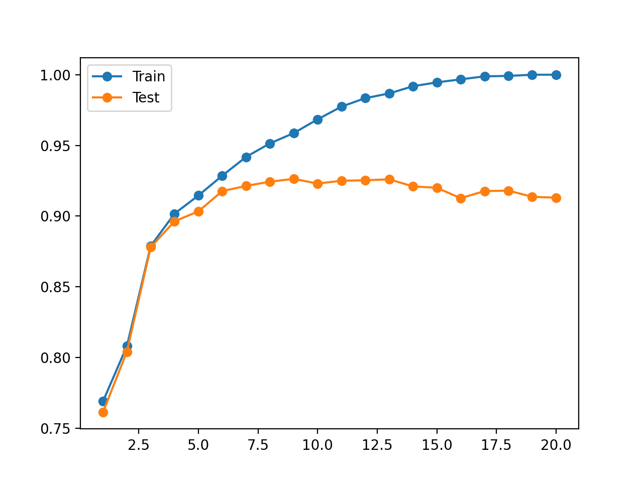
Line Plot of Decision Tree Accuracy on Train and Test Datasets for Different Tree Depths
This analysis is interesting. It shows why the model has a worse hold-out test set performance when “max_depth” is set to large values.
But it is not required.
We can just as easily choose a “max_depth” using a grid search without performing an analysis on why some values result in better performance and some result in worse performance.
In fact, in the next section, we will show where this analysis can be misleading.
Counterexample of Overfitting in Scikit-Learn
Sometimes, we may perform an analysis of machine learning model behavior and be deceived by the results.
A good example of this is varying the number of neighbors for the k-nearest neighbors algorithms, which we can implement using the KNeighborsClassifier class and configure via the “n_neighbors” argument.
Let’s forget how KNN works for the moment.
We can perform the same analysis of the KNN algorithm as we did in the previous section for the decision tree and see if our model overfits for different configuration values. In this case, we will vary the number of neighbors from 1 to 50 to get more of the effect.
The complete example is listed below.
# evaluate knn performance on train and test sets with different numbers of neighbors
from sklearn.datasets import make_classification
from sklearn.model_selection import train_test_split
from sklearn.metrics import accuracy_score
from sklearn.neighbors import KNeighborsClassifier
from matplotlib import pyplot
# create dataset
X, y = make_classification(n_samples=10000, n_features=20, n_informative=5, n_redundant=15, random_state=1)
# split into train test sets
X_train, X_test, y_train, y_test = train_test_split(X, y, test_size=0.3)
# define lists to collect scores
train_scores, test_scores = list(), list()
# define the tree depths to evaluate
values = [i for i in range(1, 51)]
# evaluate a decision tree for each depth
for i in values:
	# configure the model
	model = KNeighborsClassifier(n_neighbors=i)
	# fit model on the training dataset
	model.fit(X_train, y_train)
	# evaluate on the train dataset
	train_yhat = model.predict(X_train)
	train_acc = accuracy_score(y_train, train_yhat)
	train_scores.append(train_acc)
	# evaluate on the test dataset
	test_yhat = model.predict(X_test)
	test_acc = accuracy_score(y_test, test_yhat)
	test_scores.append(test_acc)
	# summarize progress
	print('>%d, train: %.3f, test: %.3f' % (i, train_acc, test_acc))
# plot of train and test scores vs number of neighbors
pyplot.plot(values, train_scores, '-o', label='Train')
pyplot.plot(values, test_scores, '-o', label='Test')
pyplot.legend()
pyplot.show()
Running the example fits and evaluates a KNN model on the train and test sets for each number of neighbors and reports the accuracy scores.
Note: Your results may vary given the stochastic nature of the algorithm or evaluation procedure, or differences in numerical precision. Consider running the example a few times and compare the average outcome.
Recall, we are looking for a pattern where performance on the test set improves and then starts to get worse, and performance on the training set continues to improve.
We do not see this pattern.
Instead, we see that accuracy on the training dataset starts at perfect accuracy and falls with almost every increase in the number of neighbors.
We also see that performance of the model on the holdout test improves to a value of about five neighbors, holds level and begins a downward trend after that.
>1, train: 1.000, test: 0.919
>2, train: 0.965, test: 0.916
>3, train: 0.962, test: 0.932
>4, train: 0.957, test: 0.932
>5, train: 0.954, test: 0.935
>6, train: 0.953, test: 0.934
>7, train: 0.952, test: 0.932
>8, train: 0.951, test: 0.933
>9, train: 0.949, test: 0.933
>10, train: 0.950, test: 0.935
>11, train: 0.947, test: 0.934
>12, train: 0.947, test: 0.933
>13, train: 0.945, test: 0.932
>14, train: 0.945, test: 0.932
>15, train: 0.944, test: 0.932
>16, train: 0.944, test: 0.934
>17, train: 0.943, test: 0.932
>18, train: 0.943, test: 0.935
>19, train: 0.942, test: 0.933
>20, train: 0.943, test: 0.935
>21, train: 0.942, test: 0.933
>22, train: 0.943, test: 0.933
>23, train: 0.941, test: 0.932
>24, train: 0.942, test: 0.932
>25, train: 0.942, test: 0.931
>26, train: 0.941, test: 0.930
>27, train: 0.941, test: 0.932
>28, train: 0.939, test: 0.932
>29, train: 0.938, test: 0.931
>30, train: 0.938, test: 0.931
>31, train: 0.937, test: 0.931
>32, train: 0.938, test: 0.931
>33, train: 0.937, test: 0.930
>34, train: 0.938, test: 0.931
>35, train: 0.937, test: 0.930
>36, train: 0.937, test: 0.928
>37, train: 0.936, test: 0.930
>38, train: 0.937, test: 0.930
>39, train: 0.935, test: 0.929
>40, train: 0.936, test: 0.929
>41, train: 0.936, test: 0.928
>42, train: 0.936, test: 0.929
>43, train: 0.936, test: 0.930
>44, train: 0.935, test: 0.929
>45, train: 0.935, test: 0.929
>46, train: 0.934, test: 0.929
>47, train: 0.935, test: 0.929
>48, train: 0.934, test: 0.929
>49, train: 0.934, test: 0.929
>50, train: 0.934, test: 0.929
A figure is also created that shows line plots of the model accuracy on the train and test sets with different numbers of neighbors.
The plots make the situation clearer. It looks as though the line plot for the training set is dropping to converge with the line for the test set. Indeed, this is exactly what is happening.
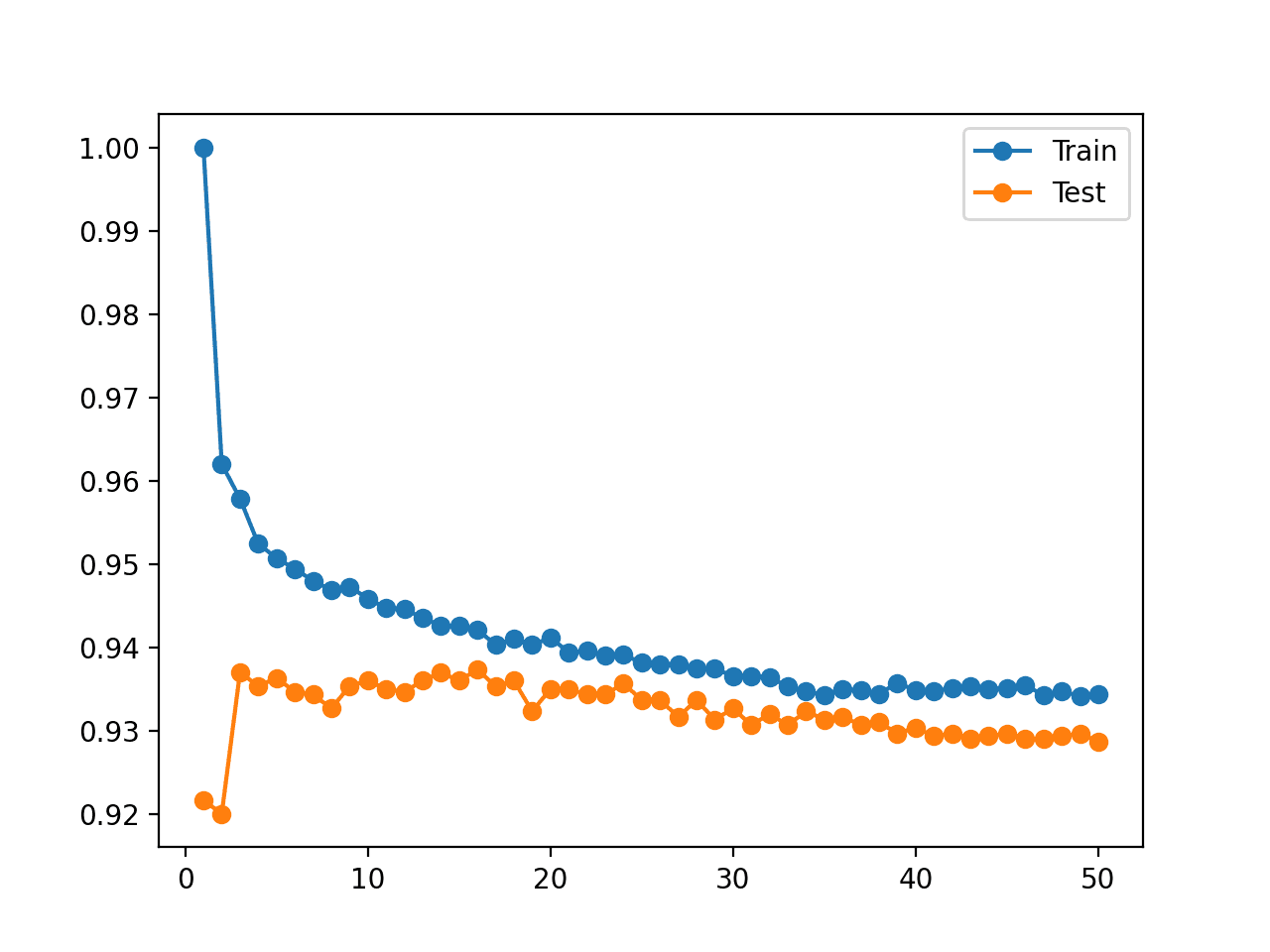
Line Plot of KNN Accuracy on Train and Test Datasets for Different Numbers of Neighbors
Now, recall how KNN works.
The “model” is really just the entire training dataset stored in an efficient data structure. Skill for the “model” on the training dataset should be 100 percent and anything less is unforgivable.
In fact, this argument holds for any machine learning algorithm and slices to the core of the confusion around overfitting for beginners.
Separate Overfitting Analysis From Model Selection
Overfitting can be an explanation for poor performance of a predictive model.
Creating learning curve plots that show the learning dynamics of a model on the train and test dataset is a helpful analysis for learning more about a model on a dataset.
But overfitting should not be confused with model selection.
We choose a predictive model or model configuration based on its out-of-sample performance. That is, its performance on new data not seen during training.
The reason we do this is that in predictive modeling, we are primarily interested in a model that makes skillful predictions. We want the model that can make the best possible predictions given the time and computational resources we have available.
This might mean we choose a model that looks like it has overfit the training dataset. In which case, an overfit analysis might be misleading.
It might also mean that the model has poor or terrible performance on the training dataset.
In general, if we cared about model performance on the training dataset in model selection, then we would expect a model to have perfect performance on the training dataset. It’s data we have available; we should not tolerate anything less.
As we saw with the KNN example above, we can achieve perfect performance on the training set by storing the training set directly and returning predictions with one neighbor at the cost of poor performance on any new data.
- Wouldn’t a model that performs well on both train and test datasets be a better model?
Maybe. But, maybe not.
This argument is based on the idea that a model that performs well on both train and test sets has a better understanding of the underlying problem.
A corollary is that a model that performs well on the test set but poor on the training set is lucky (e.g. a statistical fluke) and a model that performs well on the train set but poor on the test set is overfit.
I believe this is the sticking point for beginners that often ask how to fix overfitting for their scikit-learn machine learning model.
The worry is that a model must perform well on both train and test sets, otherwise, they are in trouble.
This is not the case.
Performance on the training set is not relevant during model selection. You must focus on the out-of-sample performance only when choosing a predictive model.
Further Reading
This section provides more resources on the topic if you are looking to go deeper.
Tutorials
- How to Avoid Overfitting in Deep Learning Neural Networks
- Overfitting and Underfitting With Machine Learning Algorithms
- How to use Learning Curves to Diagnose Machine Learning Model Performance
APIs
- sklearn.datasets.make_classification API.
- sklearn.model_selection.train_test_split API.
- sklearn.tree.DecisionTreeClassifier API.
- sklearn.neighbors.KNeighborsClassifier API.
Articles
Summary
In this tutorial, you discovered how to identify overfitting for machine learning models in Python.
Specifically, you learned:
- Overfitting is a possible cause of poor generalization performance of a predictive model.
- Overfitting can be analyzed for machine learning models by varying key model hyperparameters.
- Although overfitting is a useful tool for analysis, it must not be confused with model selection.
Do you have any questions?
Ask your questions in the comments below and I will do my best to answer.
The post How to Identify Overfitting Machine Learning Models in Scikit-Learn appeared first on Machine Learning Mastery.